
2.5: Processes and Paths
- Page ID
- 20459

\( \newcommand{\vecs}[1]{\overset { \scriptstyle \rightharpoonup} {\mathbf{#1}} } \)
\( \newcommand{\vecd}[1]{\overset{-\!-\!\rightharpoonup}{\vphantom{a}\smash {#1}}} \)
\( \newcommand{\id}{\mathrm{id}}\) \( \newcommand{\Span}{\mathrm{span}}\)
( \newcommand{\kernel}{\mathrm{null}\,}\) \( \newcommand{\range}{\mathrm{range}\,}\)
\( \newcommand{\RealPart}{\mathrm{Re}}\) \( \newcommand{\ImaginaryPart}{\mathrm{Im}}\)
\( \newcommand{\Argument}{\mathrm{Arg}}\) \( \newcommand{\norm}[1]{\| #1 \|}\)
\( \newcommand{\inner}[2]{\langle #1, #2 \rangle}\)
\( \newcommand{\Span}{\mathrm{span}}\)
\( \newcommand{\id}{\mathrm{id}}\)
\( \newcommand{\Span}{\mathrm{span}}\)
\( \newcommand{\kernel}{\mathrm{null}\,}\)
\( \newcommand{\range}{\mathrm{range}\,}\)
\( \newcommand{\RealPart}{\mathrm{Re}}\)
\( \newcommand{\ImaginaryPart}{\mathrm{Im}}\)
\( \newcommand{\Argument}{\mathrm{Arg}}\)
\( \newcommand{\norm}[1]{\| #1 \|}\)
\( \newcommand{\inner}[2]{\langle #1, #2 \rangle}\)
\( \newcommand{\Span}{\mathrm{span}}\) \( \newcommand{\AA}{\unicode[.8,0]{x212B}}\)
\( \newcommand{\vectorA}[1]{\vec{#1}} % arrow\)
\( \newcommand{\vectorAt}[1]{\vec{\text{#1}}} % arrow\)
\( \newcommand{\vectorB}[1]{\overset { \scriptstyle \rightharpoonup} {\mathbf{#1}} } \)
\( \newcommand{\vectorC}[1]{\textbf{#1}} \)
\( \newcommand{\vectorD}[1]{\overrightarrow{#1}} \)
\( \newcommand{\vectorDt}[1]{\overrightarrow{\text{#1}}} \)
\( \newcommand{\vectE}[1]{\overset{-\!-\!\rightharpoonup}{\vphantom{a}\smash{\mathbf {#1}}}} \)
\( \newcommand{\vecs}[1]{\overset { \scriptstyle \rightharpoonup} {\mathbf{#1}} } \)
\( \newcommand{\vecd}[1]{\overset{-\!-\!\rightharpoonup}{\vphantom{a}\smash {#1}}} \)
\(\newcommand{\avec}{\mathbf a}\) \(\newcommand{\bvec}{\mathbf b}\) \(\newcommand{\cvec}{\mathbf c}\) \(\newcommand{\dvec}{\mathbf d}\) \(\newcommand{\dtil}{\widetilde{\mathbf d}}\) \(\newcommand{\evec}{\mathbf e}\) \(\newcommand{\fvec}{\mathbf f}\) \(\newcommand{\nvec}{\mathbf n}\) \(\newcommand{\pvec}{\mathbf p}\) \(\newcommand{\qvec}{\mathbf q}\) \(\newcommand{\svec}{\mathbf s}\) \(\newcommand{\tvec}{\mathbf t}\) \(\newcommand{\uvec}{\mathbf u}\) \(\newcommand{\vvec}{\mathbf v}\) \(\newcommand{\wvec}{\mathbf w}\) \(\newcommand{\xvec}{\mathbf x}\) \(\newcommand{\yvec}{\mathbf y}\) \(\newcommand{\zvec}{\mathbf z}\) \(\newcommand{\rvec}{\mathbf r}\) \(\newcommand{\mvec}{\mathbf m}\) \(\newcommand{\zerovec}{\mathbf 0}\) \(\newcommand{\onevec}{\mathbf 1}\) \(\newcommand{\real}{\mathbb R}\) \(\newcommand{\twovec}[2]{\left[\begin{array}{r}#1 \\ #2 \end{array}\right]}\) \(\newcommand{\ctwovec}[2]{\left[\begin{array}{c}#1 \\ #2 \end{array}\right]}\) \(\newcommand{\threevec}[3]{\left[\begin{array}{r}#1 \\ #2 \\ #3 \end{array}\right]}\) \(\newcommand{\cthreevec}[3]{\left[\begin{array}{c}#1 \\ #2 \\ #3 \end{array}\right]}\) \(\newcommand{\fourvec}[4]{\left[\begin{array}{r}#1 \\ #2 \\ #3 \\ #4 \end{array}\right]}\) \(\newcommand{\cfourvec}[4]{\left[\begin{array}{c}#1 \\ #2 \\ #3 \\ #4 \end{array}\right]}\) \(\newcommand{\fivevec}[5]{\left[\begin{array}{r}#1 \\ #2 \\ #3 \\ #4 \\ #5 \\ \end{array}\right]}\) \(\newcommand{\cfivevec}[5]{\left[\begin{array}{c}#1 \\ #2 \\ #3 \\ #4 \\ #5 \\ \end{array}\right]}\) \(\newcommand{\mattwo}[4]{\left[\begin{array}{rr}#1 \amp #2 \\ #3 \amp #4 \\ \end{array}\right]}\) \(\newcommand{\laspan}[1]{\text{Span}\{#1\}}\) \(\newcommand{\bcal}{\cal B}\) \(\newcommand{\ccal}{\cal C}\) \(\newcommand{\scal}{\cal S}\) \(\newcommand{\wcal}{\cal W}\) \(\newcommand{\ecal}{\cal E}\) \(\newcommand{\coords}[2]{\left\{#1\right\}_{#2}}\) \(\newcommand{\gray}[1]{\color{gray}{#1}}\) \(\newcommand{\lgray}[1]{\color{lightgray}{#1}}\) \(\newcommand{\rank}{\operatorname{rank}}\) \(\newcommand{\row}{\text{Row}}\) \(\newcommand{\col}{\text{Col}}\) \(\renewcommand{\row}{\text{Row}}\) \(\newcommand{\nul}{\text{Nul}}\) \(\newcommand{\var}{\text{Var}}\) \(\newcommand{\corr}{\text{corr}}\) \(\newcommand{\len}[1]{\left|#1\right|}\) \(\newcommand{\bbar}{\overline{\bvec}}\) \(\newcommand{\bhat}{\widehat{\bvec}}\) \(\newcommand{\bperp}{\bvec^\perp}\) \(\newcommand{\xhat}{\widehat{\xvec}}\) \(\newcommand{\vhat}{\widehat{\vvec}}\) \(\newcommand{\uhat}{\widehat{\uvec}}\) \(\newcommand{\what}{\widehat{\wvec}}\) \(\newcommand{\Sighat}{\widehat{\Sigma}}\) \(\newcommand{\lt}{<}\) \(\newcommand{\gt}{>}\) \(\newcommand{\amp}{&}\) \(\definecolor{fillinmathshade}{gray}{0.9}\)
\( \newcommand{\tx}[1]{\text{#1}} % text in math mode\)
\( \newcommand{\subs}[1]{_{\text{#1}}} % subscript text\)
\( \newcommand{\sups}[1]{^{\text{#1}}} % superscript text\)
\( \newcommand{\st}{^\circ} % standard state symbol\)
\( \newcommand{\id}{^{\text{id}}} % ideal\)
\( \newcommand{\rf}{^{\text{ref}}} % reference state\)
\( \newcommand{\units}[1]{\mbox{$\thinspace$#1}}\)
\( \newcommand{\K}{\units{K}} % kelvins\)
\( \newcommand{\degC}{^\circ\text{C}} % degrees Celsius\)
\( \newcommand{\br}{\units{bar}} % bar (\bar is already defined)\)
\( \newcommand{\Pa}{\units{Pa}}\)
\( \newcommand{\mol}{\units{mol}} % mole\)
\( \newcommand{\V}{\units{V}} % volts\)
\( \newcommand{\timesten}[1]{\mbox{$\,\times\,10^{#1}$}}\)
\( \newcommand{\per}{^{-1}} % minus one power\)
\( \newcommand{\m}{_{\text{m}}} % subscript m for molar quantity\)
\( \newcommand{\CVm}{C_{V,\text{m}}} % molar heat capacity at const.V\)
\( \newcommand{\Cpm}{C_{p,\text{m}}} % molar heat capacity at const.p\)
\( \newcommand{\kT}{\kappa_T} % isothermal compressibility\)
\( \newcommand{\A}{_{\text{A}}} % subscript A for solvent or state A\)
\( \newcommand{\B}{_{\text{B}}} % subscript B for solute or state B\)
\( \newcommand{\bd}{_{\text{b}}} % subscript b for boundary or boiling point\)
\( \newcommand{\C}{_{\text{C}}} % subscript C\)
\( \newcommand{\f}{_{\text{f}}} % subscript f for freezing point\)
\( \newcommand{\mA}{_{\text{m},\text{A}}} % subscript m,A (m=molar)\)
\( \newcommand{\mB}{_{\text{m},\text{B}}} % subscript m,B (m=molar)\)
\( \newcommand{\mi}{_{\text{m},i}} % subscript m,i (m=molar)\)
\( \newcommand{\fA}{_{\text{f},\text{A}}} % subscript f,A (for fr. pt.)\)
\( \newcommand{\fB}{_{\text{f},\text{B}}} % subscript f,B (for fr. pt.)\)
\( \newcommand{\xbB}{_{x,\text{B}}} % x basis, B\)
\( \newcommand{\xbC}{_{x,\text{C}}} % x basis, C\)
\( \newcommand{\cbB}{_{c,\text{B}}} % c basis, B\)
\( \newcommand{\mbB}{_{m,\text{B}}} % m basis, B\)
\( \newcommand{\kHi}{k_{\text{H},i}} % Henry's law constant, x basis, i\)
\( \newcommand{\kHB}{k_{\text{H,B}}} % Henry's law constant, x basis, B\)
\( \newcommand{\arrow}{\,\rightarrow\,} % right arrow with extra spaces\)
\( \newcommand{\arrows}{\,\rightleftharpoons\,} % double arrows with extra spaces\)
\( \newcommand{\ra}{\rightarrow} % right arrow (can be used in text mode)\)
\( \newcommand{\eq}{\subs{eq}} % equilibrium state\)
\( \newcommand{\onehalf}{\textstyle\frac{1}{2}\D} % small 1/2 for display equation\)
\( \newcommand{\sys}{\subs{sys}} % system property\)
\( \newcommand{\sur}{\sups{sur}} % surroundings\)
\( \renewcommand{\in}{\sups{int}} % internal\)
\( \newcommand{\lab}{\subs{lab}} % lab frame\)
\( \newcommand{\cm}{\subs{cm}} % center of mass\)
\( \newcommand{\rev}{\subs{rev}} % reversible\)
\( \newcommand{\irr}{\subs{irr}} % irreversible\)
\( \newcommand{\fric}{\subs{fric}} % friction\)
\( \newcommand{\diss}{\subs{diss}} % dissipation\)
\( \newcommand{\el}{\subs{el}} % electrical\)
\( \newcommand{\cell}{\subs{cell}} % cell\)
\( \newcommand{\As}{A\subs{s}} % surface area\)
\( \newcommand{\E}{^\mathsf{E}} % excess quantity (superscript)\)
\( \newcommand{\allni}{\{n_i \}} % set of all n_i\)
\( \newcommand{\sol}{\hspace{-.1em}\tx{(sol)}}\)
\( \newcommand{\solmB}{\tx{(sol,$\,$$m\B$)}}\)
\( \newcommand{\dil}{\tx{(dil)}}\)
\( \newcommand{\sln}{\tx{(sln)}}\)
\( \newcommand{\mix}{\tx{(mix)}}\)
\( \newcommand{\rxn}{\tx{(rxn)}}\)
\( \newcommand{\expt}{\tx{(expt)}}\)
\( \newcommand{\solid}{\tx{(s)}}\)
\( \newcommand{\liquid}{\tx{(l)}}\)
\( \newcommand{\gas}{\tx{(g)}}\)
\( \newcommand{\pha}{\alpha} % phase alpha\)
\( \newcommand{\phb}{\beta} % phase beta\)
\( \newcommand{\phg}{\gamma} % phase gamma\)
\( \newcommand{\aph}{^{\alpha}} % alpha phase superscript\)
\( \newcommand{\bph}{^{\beta}} % beta phase superscript\)
\( \newcommand{\gph}{^{\gamma}} % gamma phase superscript\)
\( \newcommand{\aphp}{^{\alpha'}} % alpha prime phase superscript\)
\( \newcommand{\bphp}{^{\beta'}} % beta prime phase superscript\)
\( \newcommand{\gphp}{^{\gamma'}} % gamma prime phase superscript\)
\( \newcommand{\apht}{\small\aph} % alpha phase tiny superscript\)
\( \newcommand{\bpht}{\small\bph} % beta phase tiny superscript\)
\( \newcommand{\gpht}{\small\gph} % gamma phase tiny superscript\)
\( \newcommand{\upOmega}{\Omega}\)
\( \newcommand{\dif}{\mathop{}\!\mathrm{d}} % roman d in math mode, preceded by space\)
\( \newcommand{\Dif}{\mathop{}\!\mathrm{D}} % roman D in math mode, preceded by space\)
\( \newcommand{\df}{\dif\hspace{0.05em} f} % df\)
\(\newcommand{\dBar}{\mathop{}\!\mathrm{d}\hspace-.3em\raise1.05ex{\Rule{.8ex}{.125ex}{0ex}}} % inexact differential \)
\( \newcommand{\dq}{\dBar q} % heat differential\)
\( \newcommand{\dw}{\dBar w} % work differential\)
\( \newcommand{\dQ}{\dBar Q} % infinitesimal charge\)
\( \newcommand{\dx}{\dif\hspace{0.05em} x} % dx\)
\( \newcommand{\dt}{\dif\hspace{0.05em} t} % dt\)
\( \newcommand{\difp}{\dif\hspace{0.05em} p} % dp\)
\( \newcommand{\Del}{\Delta}\)
\( \newcommand{\Delsub}[1]{\Delta_{\text{#1}}}\)
\( \newcommand{\pd}[3]{(\partial #1 / \partial #2 )_{#3}} % \pd{}{}{} - partial derivative, one line\)
\( \newcommand{\Pd}[3]{\left( \dfrac {\partial #1} {\partial #2}\right)_{#3}} % Pd{}{}{} - Partial derivative, built-up\)
\( \newcommand{\bpd}[3]{[ \partial #1 / \partial #2 ]_{#3}}\)
\( \newcommand{\bPd}[3]{\left[ \dfrac {\partial #1} {\partial #2}\right]_{#3}}\)
\( \newcommand{\dotprod}{\small\bullet}\)
\( \newcommand{\fug}{f} % fugacity\)
\( \newcommand{\g}{\gamma} % solute activity coefficient, or gamma in general\)
\( \newcommand{\G}{\varGamma} % activity coefficient of a reference state (pressure factor)\)
\( \newcommand{\ecp}{\widetilde{\mu}} % electrochemical or total potential\)
\( \newcommand{\Eeq}{E\subs{cell, eq}} % equilibrium cell potential\)
\( \newcommand{\Ej}{E\subs{j}} % liquid junction potential\)
\( \newcommand{\mue}{\mu\subs{e}} % electron chemical potential\)
\( \newcommand{\defn}{\,\stackrel{\mathrm{def}}{=}\,} % "equal by definition" symbol\)
\( \newcommand{\D}{\displaystyle} % for a line in built-up\)
\( \newcommand{\s}{\smash[b]} % use in equations with conditions of validity\)
\( \newcommand{\cond}[1]{\\[-2.5pt]{}\tag*{#1}}\)
\( \newcommand{\nextcond}[1]{\\[-5pt]{}\tag*{#1}}\)
\( \newcommand{\R}{8.3145\units{J$\,$K$\per\,$mol$\per$}} % gas constant value\)
\( \newcommand{\Rsix}{8.31447\units{J$\,$K$\per\,$mol$\per$}} % gas constant value - 6 sig figs\)
\( \newcommand{\jn}{\hspace3pt\lower.3ex{\Rule{.6pt}{2ex}{0ex}}\hspace3pt} \)
\( \newcommand{\ljn}{\hspace3pt\lower.3ex{\Rule{.6pt}{.5ex}{0ex}}\hspace-.6pt\raise.45ex{\Rule{.6pt}{.5ex}{0ex}}\hspace-.6pt\raise1.2ex{\Rule{.6pt}{.5ex}{0ex}} \hspace3pt} \)
\( \newcommand{\lljn}{\hspace3pt\lower.3ex{\Rule{.6pt}{.5ex}{0ex}}\hspace-.6pt\raise.45ex{\Rule{.6pt}{.5ex}{0ex}}\hspace-.6pt\raise1.2ex{\Rule{.6pt}{.5ex}{0ex}}\hspace1.4pt\lower.3ex{\Rule{.6pt}{.5ex}{0ex}}\hspace-.6pt\raise.45ex{\Rule{.6pt}{.5ex}{0ex}}\hspace-.6pt\raise1.2ex{\Rule{.6pt}{.5ex}{0ex}}\hspace3pt} \)
A process is a change in the state of the system over time, starting with a definite initial state and ending with a definite final state. The process is defined by a path, which is the continuous sequence of consecutive states through which the system passes, including the initial state, the intermediate states, and the final state. The process has a direction along the path. The path could be described by a curve in an \(N\)-dimensional space in which each coordinate axis represents one of the \(N\) independent variables.
This e-book takes the view that a thermodynamic process is defined by what happens within the system, in the three-dimensional region up to and including the boundary, and by the forces exerted on the system by the surroundings and any external field. Conditions and changes in the surroundings are not part of the process except insofar as they affect these forces. For example, consider a process in which the system temperature decreases from \(300\K\) to \(273\K\). We could accomplish this temperature change by placing the system in thermal contact with either a refrigerated thermostat bath or a mixture of ice and water. The process is the same in both cases, but the surroundings are different.
Expansion is a process in which the system volume increases; in compression, the volume decreases.
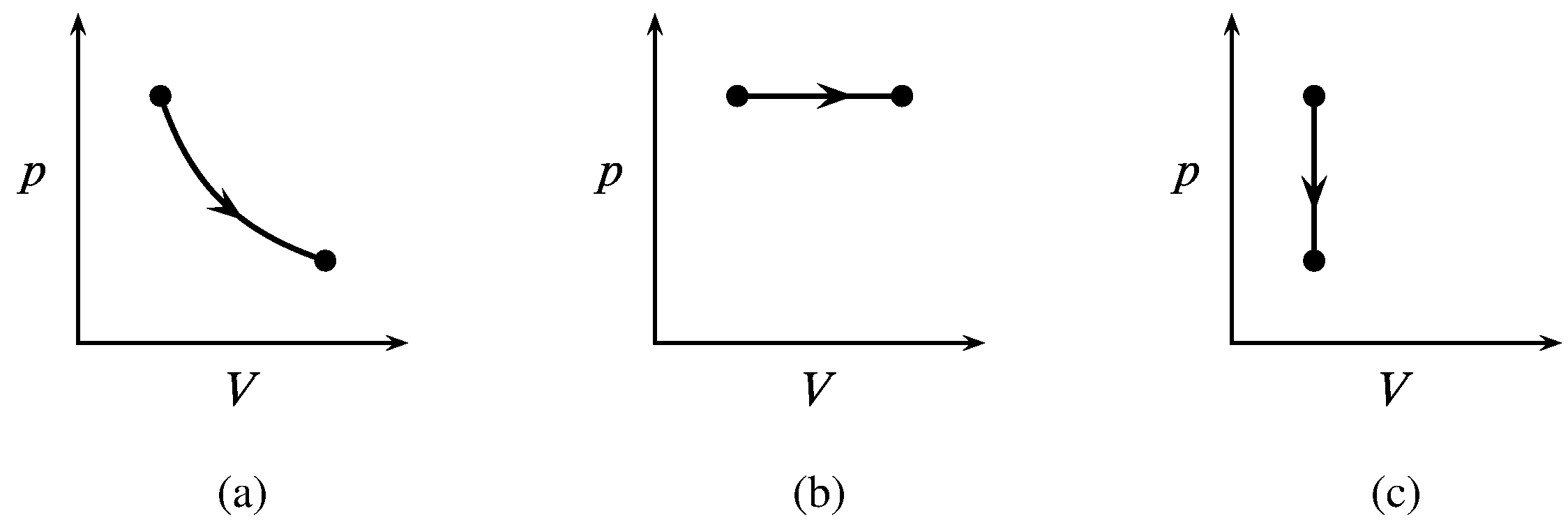
Figure 2.9 Paths of three processes of a closed ideal-gas system with \(p\) and \(V\) as the independent variables. (a) Isothermal expansion. (b) Isobaric expansion. (c) Isochoric pressure reduction.
Paths for these processes of an ideal gas are shown in Fig. 2.9. An isothermal process is one in which the temperature of the system remains uniform and constant. An isobaric or isopiestic process refers to uniform constant pressure, and an isochoric process refers to constant volume.
An adiabatic process is one in which there is no heat transfer across any portion of the boundary. We may ensure that a process is adiabatic either by using an adiabatic boundary or, if the boundary is diathermal, by continuously adjusting the external temperature to eliminate a temperature gradient at the boundary.
Recall that a state function is a property whose value at each instant depends only on the state of the system at that instant. The finite change of a state function \(X\) in a process is written \(\Del X\). The notation \(\Del X\) always has the meaning \(X_2 - X_1\), where \(X_1\) is the value in the initial state and \(X_2\) is the value in the final state. Therefore, the value of \(\Del X\) depends only on the values of \(X_1\) and \(X_2\). The change of a state function during a process depends only on the initial and final states of the system, not on the path of the process.
An infinitesimal change of the state function \(X\) is written \(\dif X\). The mathematical operation of summing an infinite number of infinitesimal changes is integration, and the sum is an integral (see the brief calculus review in Appendix E). The sum of the infinitesimal changes of \(X\) along a path is a definite integral equal to \(\Del X\): \begin{equation} \int_{X_1}^{X_2} \!\dif X = X_2-X_1 = \Delta X \tag{2.5.1} \end{equation} If \(\dif X\) obeys this relation—that is, if its integral for given limits has the same value regardless of the path—it is called an exact differential. The differential of a state function is always an exact differential.
A cyclic process is a process in which the state of the system changes and then returns to the initial state. In this case the integral of \(\dif X\) is written with a cyclic integral sign: \(\oint \dif X\). Since a state function \(X\) has the same initial and final values in a cyclic process, \(X_2\) is equal to \(X_1\) and the cyclic integral of \(\dif X\) is zero: \begin{equation} \oint \dif X = 0 \tag{2.5.2} \end{equation}
Heat (\(q\)) and work (\(w\)) are examples of quantities that are not state functions. They are not even properties of the system; instead they are quantities of energy transferred across the boundary over a period of time. It would therefore be incorrect to write “\(\Del q\)” or “\(\Del w\).” Instead, the values of \(q\) and \(w\) depend in general on the path and are called path functions.
This e-book uses the symbol \(\dBar\) (the letter “d” with a bar through the stem) for an infinitesimal quantity of a path function. Thus, \(\dq\) and \(\dw\) are infinitesimal quantities of heat and work. The sum of many infinitesimal quantities of a path function is not the difference of two values of the path function; instead, the sum is the net quantity: \begin{equation} \int \! \dq = q \qquad \int \! \dw = w \tag{2.5.3} \end{equation} The infinitesimal quantities \(\dq\) and \(\dw\), because the values of their integrals depend on the path, are inexact differentials.Chemical thermodynamicists often write these quantities as \(\dif q\) and \(\dif w\). Mathematicians, however, frown on using the same notation for inexact and exact differentials. Other notations sometimes used to indicate that heat and work are path functions are \(\tx{D}q\) and \(\tx{D}w\), and also \(\delta q\) and \(\delta w\).
There is a fundamental difference between a state function (such as temperature or volume) and a path function (such as heat or work): The value of a state function refers to one instant of time; the value of a path function refers to an interval of time.
The difference between a state function and a path function in thermodynamics is analogous to the difference between elevation and trail length in hiking up a mountain. Suppose a trailhead at the base of the mountain has several trails to the summit. The hiker at each instant is at a definite elevation above sea level. During a climb from the trailhead to the summit, the hiker’s change of elevation is independent of the trail used, but the trail length from base to summit depends on the trail.