
6.3: The Hartree-Fock Approximation
- Page ID
- 162847
\( \newcommand{\vecs}[1]{\overset { \scriptstyle \rightharpoonup} {\mathbf{#1}} } \)
\( \newcommand{\vecd}[1]{\overset{-\!-\!\rightharpoonup}{\vphantom{a}\smash {#1}}} \)
\( \newcommand{\id}{\mathrm{id}}\) \( \newcommand{\Span}{\mathrm{span}}\)
( \newcommand{\kernel}{\mathrm{null}\,}\) \( \newcommand{\range}{\mathrm{range}\,}\)
\( \newcommand{\RealPart}{\mathrm{Re}}\) \( \newcommand{\ImaginaryPart}{\mathrm{Im}}\)
\( \newcommand{\Argument}{\mathrm{Arg}}\) \( \newcommand{\norm}[1]{\| #1 \|}\)
\( \newcommand{\inner}[2]{\langle #1, #2 \rangle}\)
\( \newcommand{\Span}{\mathrm{span}}\)
\( \newcommand{\id}{\mathrm{id}}\)
\( \newcommand{\Span}{\mathrm{span}}\)
\( \newcommand{\kernel}{\mathrm{null}\,}\)
\( \newcommand{\range}{\mathrm{range}\,}\)
\( \newcommand{\RealPart}{\mathrm{Re}}\)
\( \newcommand{\ImaginaryPart}{\mathrm{Im}}\)
\( \newcommand{\Argument}{\mathrm{Arg}}\)
\( \newcommand{\norm}[1]{\| #1 \|}\)
\( \newcommand{\inner}[2]{\langle #1, #2 \rangle}\)
\( \newcommand{\Span}{\mathrm{span}}\) \( \newcommand{\AA}{\unicode[.8,0]{x212B}}\)
\( \newcommand{\vectorA}[1]{\vec{#1}} % arrow\)
\( \newcommand{\vectorAt}[1]{\vec{\text{#1}}} % arrow\)
\( \newcommand{\vectorB}[1]{\overset { \scriptstyle \rightharpoonup} {\mathbf{#1}} } \)
\( \newcommand{\vectorC}[1]{\textbf{#1}} \)
\( \newcommand{\vectorD}[1]{\overrightarrow{#1}} \)
\( \newcommand{\vectorDt}[1]{\overrightarrow{\text{#1}}} \)
\( \newcommand{\vectE}[1]{\overset{-\!-\!\rightharpoonup}{\vphantom{a}\smash{\mathbf {#1}}}} \)
\( \newcommand{\vecs}[1]{\overset { \scriptstyle \rightharpoonup} {\mathbf{#1}} } \)
\( \newcommand{\vecd}[1]{\overset{-\!-\!\rightharpoonup}{\vphantom{a}\smash {#1}}} \)
\(\newcommand{\avec}{\mathbf a}\) \(\newcommand{\bvec}{\mathbf b}\) \(\newcommand{\cvec}{\mathbf c}\) \(\newcommand{\dvec}{\mathbf d}\) \(\newcommand{\dtil}{\widetilde{\mathbf d}}\) \(\newcommand{\evec}{\mathbf e}\) \(\newcommand{\fvec}{\mathbf f}\) \(\newcommand{\nvec}{\mathbf n}\) \(\newcommand{\pvec}{\mathbf p}\) \(\newcommand{\qvec}{\mathbf q}\) \(\newcommand{\svec}{\mathbf s}\) \(\newcommand{\tvec}{\mathbf t}\) \(\newcommand{\uvec}{\mathbf u}\) \(\newcommand{\vvec}{\mathbf v}\) \(\newcommand{\wvec}{\mathbf w}\) \(\newcommand{\xvec}{\mathbf x}\) \(\newcommand{\yvec}{\mathbf y}\) \(\newcommand{\zvec}{\mathbf z}\) \(\newcommand{\rvec}{\mathbf r}\) \(\newcommand{\mvec}{\mathbf m}\) \(\newcommand{\zerovec}{\mathbf 0}\) \(\newcommand{\onevec}{\mathbf 1}\) \(\newcommand{\real}{\mathbb R}\) \(\newcommand{\twovec}[2]{\left[\begin{array}{r}#1 \\ #2 \end{array}\right]}\) \(\newcommand{\ctwovec}[2]{\left[\begin{array}{c}#1 \\ #2 \end{array}\right]}\) \(\newcommand{\threevec}[3]{\left[\begin{array}{r}#1 \\ #2 \\ #3 \end{array}\right]}\) \(\newcommand{\cthreevec}[3]{\left[\begin{array}{c}#1 \\ #2 \\ #3 \end{array}\right]}\) \(\newcommand{\fourvec}[4]{\left[\begin{array}{r}#1 \\ #2 \\ #3 \\ #4 \end{array}\right]}\) \(\newcommand{\cfourvec}[4]{\left[\begin{array}{c}#1 \\ #2 \\ #3 \\ #4 \end{array}\right]}\) \(\newcommand{\fivevec}[5]{\left[\begin{array}{r}#1 \\ #2 \\ #3 \\ #4 \\ #5 \\ \end{array}\right]}\) \(\newcommand{\cfivevec}[5]{\left[\begin{array}{c}#1 \\ #2 \\ #3 \\ #4 \\ #5 \\ \end{array}\right]}\) \(\newcommand{\mattwo}[4]{\left[\begin{array}{rr}#1 \amp #2 \\ #3 \amp #4 \\ \end{array}\right]}\) \(\newcommand{\laspan}[1]{\text{Span}\{#1\}}\) \(\newcommand{\bcal}{\cal B}\) \(\newcommand{\ccal}{\cal C}\) \(\newcommand{\scal}{\cal S}\) \(\newcommand{\wcal}{\cal W}\) \(\newcommand{\ecal}{\cal E}\) \(\newcommand{\coords}[2]{\left\{#1\right\}_{#2}}\) \(\newcommand{\gray}[1]{\color{gray}{#1}}\) \(\newcommand{\lgray}[1]{\color{lightgray}{#1}}\) \(\newcommand{\rank}{\operatorname{rank}}\) \(\newcommand{\row}{\text{Row}}\) \(\newcommand{\col}{\text{Col}}\) \(\renewcommand{\row}{\text{Row}}\) \(\newcommand{\nul}{\text{Nul}}\) \(\newcommand{\var}{\text{Var}}\) \(\newcommand{\corr}{\text{corr}}\) \(\newcommand{\len}[1]{\left|#1\right|}\) \(\newcommand{\bbar}{\overline{\bvec}}\) \(\newcommand{\bhat}{\widehat{\bvec}}\) \(\newcommand{\bperp}{\bvec^\perp}\) \(\newcommand{\xhat}{\widehat{\xvec}}\) \(\newcommand{\vhat}{\widehat{\vvec}}\) \(\newcommand{\uhat}{\widehat{\uvec}}\) \(\newcommand{\what}{\widehat{\wvec}}\) \(\newcommand{\Sighat}{\widehat{\Sigma}}\) \(\newcommand{\lt}{<}\) \(\newcommand{\gt}{>}\) \(\newcommand{\amp}{&}\) \(\definecolor{fillinmathshade}{gray}{0.9}\)Unfortunately, the Hartree approximation ignores an important property of electronic wavefunctions- their permutational antisymmetry. The full electronic Hamiltonian
\[H = \sum_j {- \dfrac{\hbar^2}{2m} \nabla^2_j - \dfrac{Ze^2}{r_j}} + \dfrac{1}{2} \sum_j^k \dfrac{e^2}{|r_j-r_k|}\label{6.1.13}\nonumber \]
is invariant (i.e., is left unchanged) under the operation \(P_{i,j}\) in which a pair of electrons have their labels (i, j) permuted. We say that \(H\) commutes with the permutation operator \(P_{i,j}\). This fact implies that any solution \(\psi\) to \(H\psi = E\psi\) must also be an eigenfunction of \(P_{i,j}\) Because permutation operators are idempotent, which means that if one applies \(P_{i,j}\) twice, one obtains the identity \(PP=1\), it can be seen that the eigenvalues of \(P_{i,j}\) must be either \(+1\) or\( –1\). That is, if \(P \psi=c\psi\), then \(P P \psi = cc \psi\), but \(PP=1\) means that \(cc = 1\), so \(c = +1\) or \(–1\).
As a result of \(H\) commuting with electron permutation operators and of the idempotency of \(P\), the eigenfunctions \(\psi\) must either be odd or even under the application of any such permutation. Particles whose wavefunctions are even under \(P\) are called Bose particles or Bosons; those for which \(\psi\) is odd are called Fermions. Electrons belong to the latter class of particles.
The simple spin-orbital product function used in Hartree theory
\[\psi= \prod_{k=1}^N \phi_k\label{6.1.14}\nonumber \]
does not have the proper permutational symmetry. For example, the Be atom function
\[\psi = 1s\alpha(1) 1s\beta(2) 2s\alpha(3) 2s\beta(4) \label{6.1.15}\nonumber \]
is not odd under the interchange of the labels of electrons 3 and 4; instead one obtains
\[P_{3,4} \psi = 1s\alpha(1) 1s\beta(2) 2s\alpha(4) 2s\beta(3) \nonumber\]
However, such products of spin-orbitals (i.e., orbitals multiplied by \(a\) or \(b\) spin functions) can be made into properly antisymmetric functions by forming the determinant of an \(N \times N\) matrix whose row index labels the spin orbital and whose column index labels the electron. For example, the Be atom function \(1s\alpha(1) 1s\beta(2) 2s\alpha(3) 2s\beta(4)\) produces the \(4 \times 4\) matrix whose determinant is shown below
\[\left|\begin{array}{cccc}
1s\alpha(1) & 1s\alpha(2) & 1s\alpha(3) & 1s\alpha(4)\\
1s\beta(1) & 1s\beta(2) & 1s\beta(3) & 1s\beta(4)\\
2s\alpha(1) & 2s\alpha(2) & 2s\alpha(3) & 2s\alpha(4)\\
2s\beta(1) & 2s\beta(2) & 2s\beta(3) & 2s\beta(4)
\end{array}\right|
\nonumber \]
Clearly, if one were to interchange any columns of this determinant, one changes the sign of the function. Moreover, if a determinant contains two or more rows that are identical (i.e., if one attempts to form such a function having two or more spin-orbitals equal), it vanishes. This is how such antisymmetric wavefunctions embody the Pauli exclusion principle.
A convenient way to write such a determinant is as follows:
\[\sum_P (-1)^p \phi_{P1} (1) \phi_{P2}(2) … \phi_{PN}(N),\nonumber \]
where the sum is over all N! permutations of the \(N\) spin-orbitals and the notation \((-1)^p\) means that a –1 is affixed to any permutation that involves an odd number of pair wise interchanges of spin-orbitals and a +1 sign is given to any that involves an even number. To properly normalize such a determinental wavefunction, one must multiply it by \(\dfrac{1}{\sqrt{N!}}\). So, the final result is that a wavefunction of the form
\[\psi = \frac{1}{\sqrt{N!}} \sum_P (-1)^p \phi_{P1} (1) \phi_{P2}(2) … \phi_{PN}(N),\label{6.1.16}\nonumber \]
which is often written in short-hand notation as,
\[\psi = |\phi_1 (1) \phi_2(2) … \phi_N(N)|\label{6.1.17}\nonumber \]
has the proper permutational antisymmetry. Note that such functions consist of as sum of \(N!\) factors, all of which have exactly the same number of electrons occupying the same spin-orbitals; the only difference among the \(N!\) terms involves which electron occupies which spin-orbital. For example, in the \(1s\alpha 2s\alpha\) function appropriate to the excited state of He, one has
\[\psi = \frac{1}{\sqrt{2}} \{1s\alpha(1) 2s\alpha(2) – 2s\alpha(1) 1s\alpha(2)\} \label{6.1.18}\nonumber \]
This function is clearly odd under the interchange of the labels of the two electrons, yet each of its two components has one electron is a \(1s\alpha\) spin-orbital and another electron in a \(2s\alpha\) spin-orbital.
Although having to make \(\psi\) antisymmetric appears to complicate matters significantly, it turns out that the Schrödinger equation appropriate to the spin-orbitals in such an antisymmetrized product wavefunction is nearly the same as the Hartree Schrödnger equation treated earlier. In fact, if one variationally minimizes the expectation value of the \(N\)-electron Hamiltonian for the above antisymmetric product wavefunction subject to the condition that the spin-orbitals are orthonormal
\[\langle\phi_J(r)| \phi_k(r)\rangle = \delta_{J,K} \label{6.1.19}\nonumber \]
one obtains the following equation for the optimal \({\phi_J(r)}\):
\[h_e \phi_J = \left[– \dfrac{\hbar^2}{2m} \nabla^2 -\dfrac{Ze^2}{r} + \sum_K \langle\phi_K(r’) | \dfrac{e^2}{|r-r’|} | \phi_K(r’)\rangle \right] \phi_J(r)\label{6.1.20}\nonumber \]
\[- \sum_K \langle\phi_K(r’) |\dfrac{e^2}{|r-r’|} | \phi_J(r’)\rangle \phi_K(r) = \epsilon_J \phi_J(r).\label{6.21}\nonumber \]
In this expression, which is known as the Hartree-Fock equation, the same kinetic and nuclear attraction potentials occur as in the Hartree equation. Moreover, the same Coulomb potential
\[\sum_K \int \phi_K(r’) \dfrac{e^2}{|r-r’|} \phi_K(r’) dr’ = \sum_K \langle\phi_K(r’)|\dfrac{e^2}{|r-r’|} |\phi_K(r’)\rangle = \sum_K J_K (r)\label{6.1.22}\nonumber \]
appears. However, one also finds a so-called exchange contribution to the Hartree-Fock potential that is equal to
\[\sum_L \langle\phi_L(r’) |\dfrac{e^2}{|r-r’|} | \phi_J(r’)\rangle \phi_L(r) \nonumber\]
and is often written in short-hand notation as \(\sum_L K_L \phi_J(r)\). Notice that the Coulomb and exchange terms cancel for the \(L=J\) case; this causes the artificial self-interaction term \(J_L \phi_L(r) \) that can appear in the Hartree equations (unless one explicitly eliminates it) to automatically cancel with the exchange term \(K_L \phi_L(r)\) in the Hartree-Fock equations.
To derive the above Hartree-Fock equations, one must make use of the so-called Slater-Condon rules to express the Hamiltonian expectation value as
\[ \langle|\phi_1(1)\phi_2(2)\cdots \phi_{N-1}\phi_N(N)|H|\phi_1(1)\phi_2(2)\cdots \phi_{N-1}\phi_N(N)|\rangle =\sum_{j=1}^N\langle\phi_j(r)|-\frac{1}{2}\nabla^2-\frac{e^2}{r}|\phi_j(r)\rangle \\+\frac{1}{2}\sum_{j,k=1}^N\left[ \langle\phi_j(r)\phi_k(r')|\frac{e^2}{|r-r'|}|\phi_j(r)\phi_k(r')\rangle
- \langle\phi_j(r)\phi_k(r')|\frac{e^2}{|r-r'|}|\phi_k(r)\phi_j(r')\rangle\right]\nonumber \]
This expectation value is a sum of terms (the kinetic energy and electron-nuclear Coulomb potentials) that vary quadratically on the spin-orbitals (i.e., as \(\langle \phi| {\rm operator} |\phi\rangle\)) plus another sum (the Coulomb and exchange electron-electron interaction terms) that depend on the fourth power of the spin-orbitals (i.e., as \(\langle \phi\phi |{\rm operator} |\phi\phi \rangle\). When these terms are differentiated to minimize the expectation value, they generate factors that scale linearly and with the third power of the spin-orbitals. These are the factors
\[{-\dfrac{\hbar^2}{2m} \nabla^2 -\frac{Z_e^2}{r} } \phi_J(r)\nonumber \] and \[\sum_K \langle\phi_K(r’) |\frac{e^2}{|r-r’|} | \phi_K(r’)\rangle \phi_J(r) - \sum_K \langle \phi_K(r’) |\frac{e^2}{|r-r’|} | \phi_J(r’)\rangle \phi_K(r) \label{6.1.23}\]
appearing in the Hartree-Fock equations shown above.
When the LCAO expansion of each Hartree-Fock (HF) spin-orbital is substituted into the above HF Schrödinger equation, a matrix equation is again obtained:
\[\sum_\mu \langle\chi_\nu |h_e| \chi_\mu\rangle C_{J,\mu} = \epsilon_J \sum_\mu \langle\chi_\nu|\chi_\mu\rangle C_{J,\mu}\label{6.1.24}\nonumber \]
where the overlap integral \(\langle\chi_\nu|\chi_\mu\rangle\) is as defined earlier, and the \(h_e\) matrix element is
\[\langle\chi_\nu| h_e| \chi_\mu\rangle = \langle\chi_\nu| -\dfrac{\hbar^2}{2m} \nabla^2 |\chi_\mu\rangle + \langle\chi_\nu| -\frac{Ze^2}{r} |\chi_\mu\rangle \label{6.1.25}\]
\[+ \sum_{K,\eta,\gamma} C_{K,\eta} C_{K,\gamma} [\langle\chi_\nu(r) \chi_\eta(r’) |\frac{e^2}{|r-r’|} | \chi_\mu(r) \chi_\gamma(r’)\rangle - \langle\chi_\nu(r) \chi_\eta(r’) |\frac{e^2}{|r-r’|} | \chi_\gamma(r) \chi_\mu (r’)\rangle].\label{6.1.26}\]
Clearly, the only difference between this expression and the corresponding result of Hartree theory is the presence of the last term, the exchange integral. The SCF iterative procedure used to solve the Hartree equations is again used to solve the HF equations.
It is useful to reflect on the physical meaning of the Coulomb and exchange interactions between pairs of orbitals. For example, the Coulomb integral
\[ J_{1,2} = \int |\phi_1(r)|^2 \frac{e^2}{|r-r’|} |\phi_2(r’)|^2 dr dr’ \label{6.1.27}\nonumber \]
appropriate to the two orbitals shown in Figure 6.1.3 represents the Coulombic repulsion energy \(\dfrac{e^2}{|r-r’|}\) of two charge densities, \(|\phi_1|^2\) and \(|\phi_2|^2\), integrated over all locations \(r\) and \(r’\) of the two electrons.
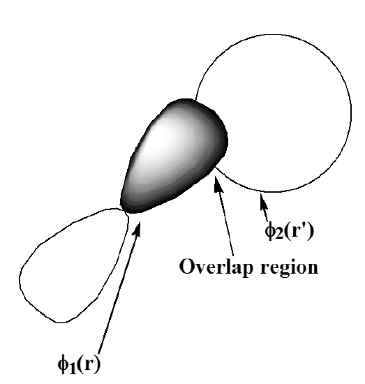
In contrast, the exchange integral
\[K_{1,2} = \int \phi_1(r) \phi_2(r’) \frac{e^2}{|r-r’|} \phi_2(r) \phi_1(r’) dr dr’\label{6.1.28}\nonumber \]
can be thought of as the Coulombic repulsion between two electrons whose coordinates \(r\) and \(r’\) are both distributed throughout the “overlap region” \(\phi_1\) \(\phi_2\). This overlap region is where both \(\phi_1\) and \(\phi_2\) have appreciable magnitude, so exchange integrals tend to be significant in magnitude only when the two orbitals involved have substantial regions of overlap.
Finally, a few words are in order about one of the most computer time-consuming parts of any Hartree-Fock calculation (or those discussed later)- the task of evaluating and transforming the two-electron integrals
\[\langle\chi_\nu(r) \chi_\eta(r’) |\frac{e^2}{|r-r’|} | \chi_\mu(r) \chi_\gamma(r’)\rangle.\label{6.1.29}\nonumber \]
When M GTOs are used as basis functions, the evaluation of \(\dfrac{M^4}{8}\) of these integrals often poses a major hurdle. For example, with 500 basis orbitals, there will be of the order of 7.8 x10⁹ such integrals. With each integral requiring 2 words of disk storage (most integrals need to be evaluated in double precision), this would require at least 1.5 x10⁴ Mwords of disk storage. Even in the era of modern computers that possess 500 Gby disks, this is a significant requirement. One of the more important technical advances that is under much current development is the efficient calculation of such integrals when the product functions \(\chi_\nu(r) \chi_\mu(r)\) and \(\chi_\gamma(r’) \chi_\eta(r’)\) that display the dependence on the two electrons’ coordinates r and r’ are spatially distant. In particular, so-called multipole expansions of these product functions are used to obtain more efficient approximations to their integrals when these functions are far apart. Moreover, such expansions offer a reliable way to ignore (i.e., approximate as zero) many integrals whose product functions are sufficiently distant. Such approaches show considerable promise for reducing the \(\dfrac{M^4}{8}\) two-electron integral list to one whose size scales much less strongly with the size of the AO basis and form an important component if efforts to achieve CPU and storage needs that scale linearly with the size of the molecule.
Koopmans’ Theorem
The HF-SCF equations \(h_e \phi_i = \epsilon_i \phi_i\) imply that the orbital energies \(\epsilon_i\) can be written as:
\[\epsilon_i = \langle \phi_i | h_e | \phi_i \rangle = \langle \phi_i | T + V | \phi_i \rangle + \sum_{j({\rm occupied})} \langle \phi_i | J_j - K_j | \phi_i \rangle \nonumber \]
\[= \langle \phi_i | T + V | \phi_i \rangle + \sum_{j({\rm occupied})} [ J_{i,j} - K_{i,j} ],\label{6.1.30}\nonumber \]
where \(T + V\) represents the kinetic (\(T\)) and nuclear attraction (\(V\)) energies, respectively. Thus, \(\epsilon_i\) is the average value of the kinetic energy plus Coulombic attraction to the nuclei for an electron in \(\phi_i\) plus the sum over all of the spin-orbitals occupied in \(\psi\) of Coulomb minus Exchange interactions of these electrons with the electron in \(\phi_i\).
If \(\phi_i\) is an occupied spin-orbital, the \(j = i\) term \([ J_{i,i} - K_{i,i}]\) disappears in the above sum and the remaining terms in the sum represent the Coulomb minus exchange interaction of \(\phi_i\) with all of the \(N-1\) other occupied spin-orbitals. If \(\phi_i\) is a virtual spin-orbital, this cancelation does not occur because the sum over \(j\) does not include \(j = i\). So, one obtains the Coulomb minus exchange interaction of \(\phi_i\) with all \(N\) of the occupied spin-orbitals in \(\psi\). Hence the energies of occupied orbitals pertain to interactions appropriate to a total of \(N\) electrons, while the energies of virtual orbitals pertain to a system with \(N+1\) electrons. This difference is very important to understand and to keep in mind.
Let us consider the following model of the detachment or attachment of an electron in an \(N\)-electron system.
- In this model, both the parent molecule and the species generated by adding or removing an electron are treated at the single-determinant level.
- The Hartree-Fock orbitals of the parent molecule are used to describe both species. It is said that such a model neglects orbital relaxation (i.e., the re-optimization of the spin-orbitals to allow them to become appropriate to the daughter species).
Within this model, the energy difference between the daughter and the parent can be written as follows (\(\phi_k\) represents the particular spin-orbital that is added or removed):
for electron detachment:
\[E_{N-1} - E_N = - \epsilon_k \label{6.1.31}\nonumber \]
and for electron attachment:
\[E_N - E_{N+1} = - \epsilon_k .\label{6.1.32}\nonumber \]
Let’s derive this result for the case in which an electron is added to the \(N+1^{st}\) spin-orbital. Again, using the Slater-Condon rules from Section 6.1.2 of this Chapter, the energy of the \(N\)-electron determinant with spin-orbitals \(\phi_1\) through \(f_N\) occupied is
\[E_N = \sum_{i=1}^N \langle \phi_i | T + V | \phi_i \rangle + \sum_{i=1}^{N} [ J_{i,j} - K_{i,j} ],\label{6.1.33}\nonumber \]
which can also be written as
\[E_N = \sum_{i=1}^N \langle \phi_i | T + V | \phi_i \rangle + \frac{1}{2} \sum_{i,j=1}^{N} [ J_{i,j} - K_{i,j} ].\label{6.1.34}\nonumber \]
Likewise, the energy of the \(N+1\)-electron determinant wavefunction is
\[E_{N+1} = \sum_{i=1}^{N+1} \langle \phi_i | T + V | \phi_i \rangle + \frac{1}{2} \sum_{i,j=1}^{N+1} [ J_{i,j} - K_{i,j} ].\label{6.1.35}\nonumber \]
The difference between these two energies is given by
\[E_{N} – E_{N+1} = - \langle \phi_{N+1} | T + V | \phi_{N+1} \rangle - \frac{1}{2} \sum_{i=1}^{N+1} [ J_{i,N+1} - K_{i,N+1} ]\label{6.1.36}\nonumber \]
\[- \frac{1}{2} \sum_{j=1}^{N+1} [ J_{N+1,j} - K_{N+1,j} ] = - \langle \phi_{N+1} | T + V | \phi_{N+1} \rangle - \sum_{i=1}^{N+1} [ J_{i,N+1} - K_{i,N+1} ]\label{6.1.37}\nonumber \]
\[= - \epsilon_{N+1}.\label{6.1.38}\nonumber \]
That is, the energy difference is equal to minus the expression for the energy of the \(N+1^{st}\) spin-orbital, which was given earlier.
So, within the limitations of the HF, frozen-orbital model, the ionization potentials (IPs) and electron affinities (EAs) are given as the negative of the occupied and virtual spin-orbital energies, respectively. This statement is referred to as Koopmans’ theorem; it is used extensively in quantum chemical calculations as a means of estimating IPs and EAs and often yields results that are qualitatively correct (i.e., ± 0.5 eV).
Orbital Energies and the Total Energy
The total HF-SCF electronic energy can be written as:
\[E = \sum_{i({\rm occupied})} \langle \phi_i | T + V | \phi_i \rangle + \sum_{i>j_{({\rm occupied})}} [ J_{i,j} - K_{i,j} ] \label{6.1.39}\nonumber \]
and the sum of the orbital energies of the occupied spin-orbitals is given by:
\[\sum_{i({\rm occupied})} \epsilon_i = \sum_{i({\rm occupied})} \langle \phi_i | T + V | \phi_i \rangle + \sum_{i,j({\rm occupied})} [J_{i,j} - K_{i,j} ]. \label{6.1.40}\nonumber \]
These two expressions differ in a very important way; the sum of occupied orbital energies double counts the Coulomb minus exchange interaction energies. Thus, within the Hartree-Fock approximation, the sum of the occupied orbital energies is not equal to the total energy. This finding teaches us that we can not think of the total electronic energy of a given orbital occupation in terms of the orbital energies alone. We need to also keep track of the inter-electron Coulomb and Exchange energies.