
2.4: Hückel or Tight Binding Theory
- Page ID
- 17181

\( \newcommand{\vecs}[1]{\overset { \scriptstyle \rightharpoonup} {\mathbf{#1}} } \)
\( \newcommand{\vecd}[1]{\overset{-\!-\!\rightharpoonup}{\vphantom{a}\smash {#1}}} \)
\( \newcommand{\id}{\mathrm{id}}\) \( \newcommand{\Span}{\mathrm{span}}\)
( \newcommand{\kernel}{\mathrm{null}\,}\) \( \newcommand{\range}{\mathrm{range}\,}\)
\( \newcommand{\RealPart}{\mathrm{Re}}\) \( \newcommand{\ImaginaryPart}{\mathrm{Im}}\)
\( \newcommand{\Argument}{\mathrm{Arg}}\) \( \newcommand{\norm}[1]{\| #1 \|}\)
\( \newcommand{\inner}[2]{\langle #1, #2 \rangle}\)
\( \newcommand{\Span}{\mathrm{span}}\)
\( \newcommand{\id}{\mathrm{id}}\)
\( \newcommand{\Span}{\mathrm{span}}\)
\( \newcommand{\kernel}{\mathrm{null}\,}\)
\( \newcommand{\range}{\mathrm{range}\,}\)
\( \newcommand{\RealPart}{\mathrm{Re}}\)
\( \newcommand{\ImaginaryPart}{\mathrm{Im}}\)
\( \newcommand{\Argument}{\mathrm{Arg}}\)
\( \newcommand{\norm}[1]{\| #1 \|}\)
\( \newcommand{\inner}[2]{\langle #1, #2 \rangle}\)
\( \newcommand{\Span}{\mathrm{span}}\) \( \newcommand{\AA}{\unicode[.8,0]{x212B}}\)
\( \newcommand{\vectorA}[1]{\vec{#1}} % arrow\)
\( \newcommand{\vectorAt}[1]{\vec{\text{#1}}} % arrow\)
\( \newcommand{\vectorB}[1]{\overset { \scriptstyle \rightharpoonup} {\mathbf{#1}} } \)
\( \newcommand{\vectorC}[1]{\textbf{#1}} \)
\( \newcommand{\vectorD}[1]{\overrightarrow{#1}} \)
\( \newcommand{\vectorDt}[1]{\overrightarrow{\text{#1}}} \)
\( \newcommand{\vectE}[1]{\overset{-\!-\!\rightharpoonup}{\vphantom{a}\smash{\mathbf {#1}}}} \)
\( \newcommand{\vecs}[1]{\overset { \scriptstyle \rightharpoonup} {\mathbf{#1}} } \)
\( \newcommand{\vecd}[1]{\overset{-\!-\!\rightharpoonup}{\vphantom{a}\smash {#1}}} \)
\(\newcommand{\avec}{\mathbf a}\) \(\newcommand{\bvec}{\mathbf b}\) \(\newcommand{\cvec}{\mathbf c}\) \(\newcommand{\dvec}{\mathbf d}\) \(\newcommand{\dtil}{\widetilde{\mathbf d}}\) \(\newcommand{\evec}{\mathbf e}\) \(\newcommand{\fvec}{\mathbf f}\) \(\newcommand{\nvec}{\mathbf n}\) \(\newcommand{\pvec}{\mathbf p}\) \(\newcommand{\qvec}{\mathbf q}\) \(\newcommand{\svec}{\mathbf s}\) \(\newcommand{\tvec}{\mathbf t}\) \(\newcommand{\uvec}{\mathbf u}\) \(\newcommand{\vvec}{\mathbf v}\) \(\newcommand{\wvec}{\mathbf w}\) \(\newcommand{\xvec}{\mathbf x}\) \(\newcommand{\yvec}{\mathbf y}\) \(\newcommand{\zvec}{\mathbf z}\) \(\newcommand{\rvec}{\mathbf r}\) \(\newcommand{\mvec}{\mathbf m}\) \(\newcommand{\zerovec}{\mathbf 0}\) \(\newcommand{\onevec}{\mathbf 1}\) \(\newcommand{\real}{\mathbb R}\) \(\newcommand{\twovec}[2]{\left[\begin{array}{r}#1 \\ #2 \end{array}\right]}\) \(\newcommand{\ctwovec}[2]{\left[\begin{array}{c}#1 \\ #2 \end{array}\right]}\) \(\newcommand{\threevec}[3]{\left[\begin{array}{r}#1 \\ #2 \\ #3 \end{array}\right]}\) \(\newcommand{\cthreevec}[3]{\left[\begin{array}{c}#1 \\ #2 \\ #3 \end{array}\right]}\) \(\newcommand{\fourvec}[4]{\left[\begin{array}{r}#1 \\ #2 \\ #3 \\ #4 \end{array}\right]}\) \(\newcommand{\cfourvec}[4]{\left[\begin{array}{c}#1 \\ #2 \\ #3 \\ #4 \end{array}\right]}\) \(\newcommand{\fivevec}[5]{\left[\begin{array}{r}#1 \\ #2 \\ #3 \\ #4 \\ #5 \\ \end{array}\right]}\) \(\newcommand{\cfivevec}[5]{\left[\begin{array}{c}#1 \\ #2 \\ #3 \\ #4 \\ #5 \\ \end{array}\right]}\) \(\newcommand{\mattwo}[4]{\left[\begin{array}{rr}#1 \amp #2 \\ #3 \amp #4 \\ \end{array}\right]}\) \(\newcommand{\laspan}[1]{\text{Span}\{#1\}}\) \(\newcommand{\bcal}{\cal B}\) \(\newcommand{\ccal}{\cal C}\) \(\newcommand{\scal}{\cal S}\) \(\newcommand{\wcal}{\cal W}\) \(\newcommand{\ecal}{\cal E}\) \(\newcommand{\coords}[2]{\left\{#1\right\}_{#2}}\) \(\newcommand{\gray}[1]{\color{gray}{#1}}\) \(\newcommand{\lgray}[1]{\color{lightgray}{#1}}\) \(\newcommand{\rank}{\operatorname{rank}}\) \(\newcommand{\row}{\text{Row}}\) \(\newcommand{\col}{\text{Col}}\) \(\renewcommand{\row}{\text{Row}}\) \(\newcommand{\nul}{\text{Nul}}\) \(\newcommand{\var}{\text{Var}}\) \(\newcommand{\corr}{\text{corr}}\) \(\newcommand{\len}[1]{\left|#1\right|}\) \(\newcommand{\bbar}{\overline{\bvec}}\) \(\newcommand{\bhat}{\widehat{\bvec}}\) \(\newcommand{\bperp}{\bvec^\perp}\) \(\newcommand{\xhat}{\widehat{\xvec}}\) \(\newcommand{\vhat}{\widehat{\vvec}}\) \(\newcommand{\uhat}{\widehat{\uvec}}\) \(\newcommand{\what}{\widehat{\wvec}}\) \(\newcommand{\Sighat}{\widehat{\Sigma}}\) \(\newcommand{\lt}{<}\) \(\newcommand{\gt}{>}\) \(\newcommand{\amp}{&}\) \(\definecolor{fillinmathshade}{gray}{0.9}\)Now, let’s examine what determines the energy range into which orbitals (e.g., \(p_\pi\) orbitals in polyenes, metal, semi-conductor, or insulator; \(\sigma\) or \(p_\sigma\) orbitals in a solid; or \(\sigma\) or \(\pi\) atomic orbitals in a molecule) split. I know that, in our earlier discussion, we talked about the degree of overlap between orbitals on neighboring atoms relating to the energy splitting, but now it is time to make this concept more quantitative. To begin, consider two orbitals, one on an atom labeled A and another on a neighboring atom labeled B; these orbitals could be, for example, the \(1s\) orbitals of two hydrogen atoms, such as Figure 2.9 illustrates.
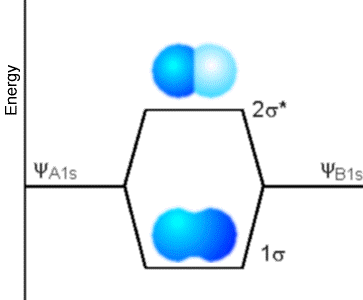
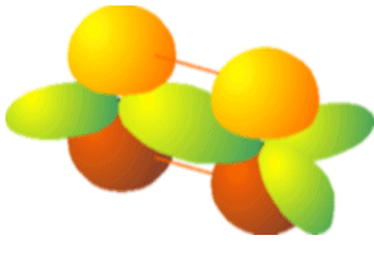
However, the two orbitals could instead be two \(p_\pi\) orbitals on neighboring carbon atoms such as are shown in Figure 2.10 as they form \(\pi\) bonding and \(\pi^*\) anti-bonding orbitals.
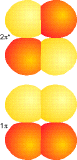
Figure 2.10. Two atomic \(p_\pi\) orbitals form a bonding \(\pi\) and antibonding \(\pi^*\) molecular orbital.
In both of these cases, we think of forming the molecular orbitals (MOs) \(\phi_k\) as linear combinations of the atomic orbitals (AOs) ca on the constituent atoms, and we express this mathematically as follows:
\[\phi_K = \sum_a C_{K,a} \chi_a,\]
where the \(C_{K,a}\) are called linear combination of atomic orbital to form molecular orbital (LCAO-MO) coefficients. The MOs are supposed to be solutions to the Schrödinger equation in which the Hamiltonian H involves the kinetic energy of the electron as well as the potentials \(V_L\) and \(V_R\) detailing its attraction to the left and right atomic centers (this one-electron Hamiltonian is only an approximation for describing molecular orbitals; more rigorous N-electron treatments will be discussed in Chapter 6):
\[H = - \dfrac{\hbar^2}{2m} \nabla^2 + V_L + V_R.\]
In contrast, the AOs centered on the left atom A are supposed to be solutions of the Schrödinger equation whose Hamiltonian is \(H = - \dfrac{\hbar^2}{2m} \nabla^2 + V_L\), and the AOs on the right atom B have \(H = - \dfrac{\hbar^2}{2m} \nabla^2 + V_R\). Substituting \(\phi_K = \sum_a C_{K,a} \chi_a\) into the MO’s Schrödinger equation
\[\textbf{H}\phi_K = \varepsilon_K \phi_K\]
and then multiplying on the left by the complex conjugate of \(\chi_b\) and integrating over the \(r\), \(\theta\) and \(\phi\) coordinates of the electron produces
\[\sum_a \langle \chi_b| - \dfrac{\hbar^2}{2m} \nabla^2 + V_L + V_R |\chi_a\rangle C_{K,a} = \varepsilon_K \sum_a \langle \chi_b|\chi_a\rangle C_{K,a}\]
Recall that the Dirac notation \(\langle a|b\rangle\) denotes the integral of \(a^*\) and \(b\), and \(\langle a| op| b\rangle\) denotes the integral of \(a^*\) and the operator op acting on b.
In what is known as the Hückel model in chemistry or the tight-binding model in solid-state theory, one approximates the integrals entering into the above set of linear equations as follows:
- The diagonal integral \(\langle \chi_b| - \dfrac{\hbar^2}{2m} \nabla^2 + V_L + V_R |\chi_b\rangle \) involving the AO centered on the right atom and labeled \(\chi_b\) is assumed to be equivalent to \(\langle \chi_b| - \dfrac{\hbar^2}{2m} \nabla^2 + V_R |\chi_b\rangle \), which means that net attraction of this orbital to the left atomic center is neglected. Moreover, this integral is approximated in terms of the binding energy (denoted \(\alpha\), not to be confused with the electron spin function a) for an electron that occupies the \(\chi_b\) orbital: \(\langle \chi_b| - \dfrac{\hbar^2}{2m} \nabla^2 + V_R |\chi_b\rangle = \alpha_b \). The physical meaning of \(\alpha_b\) is the kinetic energy of the electron in \(\chi_b\) plus the attraction of this electron to the right atomic center while it resides in \(\chi_b\). Of course, an analogous approximation is made for the diagonal integral involving \(\chi_a\); \(\langle \chi_a| - \dfrac{\hbar^2}{2m} \nabla^2 + V_L |\chi_a\rangle = \alpha_a \) . These \(\alpha\) values are negative quantities because, as is convention in electronic structure theory, energies are measured relative to the energy of the electron when it is removed from the orbital and possesses zero kinetic energy.
- The off-diagonal integrals \(\langle \chi_b| - \dfrac{\hbar^2}{2m} \nabla^2 + V_L + V_R |\chi_a\rangle \) are expressed in terms of a parameter \(\beta_{a,b}\) which relates to the kinetic and potential energy of the electron while it resides in the “overlap region” in which both \(\chi_a\) and \(\chi_b\) are non-vanishing. This region is shown pictorially above as the region where the left and right orbitals touch or overlap. The magnitude of \(\beta\) is assumed to be proportional to the overlap \(S_{a,b}\) between the two AOs : \(S_{a,b} = \langle \chi_a|\chi_b\rangle \). It turns out that \(\beta\) is usually a negative quantity, which can be seen by writing it as \(\langle \chi_b| - \dfrac{\hbar^2}{2m} \nabla^2 + V_R |\chi_a\rangle + \langle \chi_b| V_L |\chi_a\rangle \). Since \(\chi_a\) is an eigenfunction of \(- \dfrac{\hbar^2}{2m} \nabla^2 + V_R\) having the eigenvalue \(\alpha_a\), the first term is equal to \(\alpha_a\) (a negative quantity) times \(\langle \chi_b|\chi_a\rangle \), the overlap \(S\). The second quantity \(\langle \chi_b| V_L |\chi_a\rangle \) is equal to the integral of the overlap density \(\chi_b(r)\chi_a(r)\) multiplied by the (negative) Coulomb potential for attractive interaction of the electron with the left atomic center. So, whenever \(\chi_b(r)\) and \(\chi_a(r)\) have positive overlap, b will turn out negative.
iii. Finally, in the most elementary Hückel or tight-binding model, the off-diagonal overlap integrals \(\langle \chi_a|\chi_b\rangle =S_{a,b}\) are neglected and set equal to zero on the right side of the matrix eigenvalue equation. However, in some Hückel models, overlap between neighboring orbitals is explicitly treated, so, in some of the discussion below we will retain \(S_{a,b}\).
With these Hückel approximations, the set of equations that determine the orbital energies \(\varepsilon_K\) and the corresponding LCAO-MO coefficients \(C_{K,a}\) are written for the two-orbital case at hand as in the first \(2\times2\) matrix equations shown below
\[
\left[ \begin{array}{cc}
\alpha & \beta \\
\beta & \alpha
\end{array}
\right]
\left[\begin{array}{c}
C_L\\
C_R
\end{array}
\right]
=\varepsilon
\left[ \begin{array}{cc}
1 & S \\
S & 1
\end{array}
\right]
\left[\begin{array}{c}
C_L\\
C_R
\end{array}
\right]
\]
which is sometimes written a
\[
\left[ \begin{array}{cc}
\alpha-\varepsilon & \beta-\varepsilon S \\
\beta-\varepsilon S & \alpha-\varepsilon
\end{array}
\right]
\left[\begin{array}{c}
C_L\\
C_R
\end{array}
\right]
=
\left[\begin{array}{c}
0\\
0
\end{array}
\right]
\]
These equations reduce with the assumption of zero overlap to
\[
\left[ \begin{array}{cc}
\alpha & \beta \\
\beta & \alpha
\end{array}
\right]
\left[\begin{array}{c}
C_L\\
C_R
\end{array}
\right]
=\varepsilon
\left[ \begin{array}{cc}
1 & 0 \\
0 & 1
\end{array}
\right]
\left[\begin{array}{c}
C_L\\
C_R
\end{array}
\right]
\]
The a parameters are identical if the two AOs ca and \(\chi_b\) are identical, as would be the case for bonding between the two \(1s\) orbitals of two H atoms or two 2\(p_\pi\) orbitals of two C atoms or two 3s orbitals of two Na atoms. If the left and right orbitals were not identical (e.g., for bonding in HeH+ or for the \(\pi\) bonding in a C-O group), their a values would be different and the Hückel matrix problem would look like:
\[
\left[ \begin{array}{cc}
\alpha & \beta \\
\beta & \alpha'
\end{array}
\right]
\left[\begin{array}{c}
C_L\\
C_R
\end{array}
\right]
=\varepsilon
\left[ \begin{array}{cc}
1 & S \\
S & 1
\end{array}
\right]
\left[\begin{array}{c}
C_L\\
C_R
\end{array}
\right]
\]
To find the MO energies that result from combining the AOs, one must find the values of e for which the above equations are valid. Taking the \(2\times2\) matrix consisting of e times the overlap matrix to the left hand side, the above set of equations reduces to the third set displayed earlier. It is known from matrix algebra that such a set of linear homogeneous equations (i.e., having zeros on the right hand sides) can have non-trivial solutions (i.e., values of \(C\) that are not simply zero) only if the determinant of the matrix on the left side vanishes. Setting this determinant equal to zero gives a quadratic equation in which the e values are the unknowns:
\[(\alpha-\varepsilon)^2 – (\beta - \varepsilon S)^2 = 0.\]
This quadratic equation can be factored into a product
\[(\alpha - \beta - \varepsilon +\varepsilon S) (\alpha + \beta - \varepsilon -\varepsilon S) = 0\]
which has two solutions
\[\varepsilon = \frac{\alpha + \beta}{1 + S}, \text{ and } \varepsilon = \frac{\alpha - \beta}{1 – S}.\]
As discussed earlier, it turns out that the b values are usually negative, so the lowest energy such solution is the \(\varepsilon = (\alpha + \beta)/(1 + S)\) solution, which gives the energy of the bonding MO. Notice that the energies of the bonding and anti-bonding MOs are not symmetrically displaced from the value a within this version of the Hückel model that retains orbital overlap. In fact, the bonding orbital lies less than b below a, and the antibonding MO lies more than b above a because of the \(1+S\) and \(1-S\) factors in the respective denominators. This asymmetric lowering and raising of the MOs relative to the energies of the constituent AOs is commonly observed in chemical bonds; that is, the antibonding orbital is more antibonding than the bonding orbital i\(\sigma\) bonding. This is another important thing to keep in mind because its effects pervade chemical bonding and spectroscopy.
Having noted the effect of inclusion of AO overlap effects in the Hückel model, I should admit that it is far more common to utilize the simplified version of the Hückel model in which the S factors are ignored. In so doing, one obtains patterns of MO orbital energies that do not reflect the asymmetric splitting in bonding and antibonding orbitals noted above. However, this simplified approach is easier to use and offers qualitatively correct MO energy orderings. So, let’s proceed with our discussion of the Hückel model in its simplified version.
To obtain the LCAO-MO coefficients corresponding to the bonding and antibonding MOs, one substitutes the corresponding a values into the linear equations
\[
\left[ \begin{array}{cc}
\alpha-\varepsilon & \beta \\
\beta & \alpha-\varepsilon
\end{array}
\right]
\left[\begin{array}{c}
C_L\\
C_R
\end{array}
\right]
=
\left[\begin{array}{c}
0\\
0
\end{array}
\right]
\]
and solves for the \(C_a\) coefficients (actually, one can solve for all, but one \(C_a\), and then use normalization of the MO to determine the final Ca). For example, for the bonding MO, we substitute \(\varepsilon = \alpha + \beta\) into the above matrix equation and obtain two equations for \(C_L\) and \(C_R\):
\[- \beta C_L + \beta C_R = 0\]
\[\beta C_L - \beta C_R = 0.\]
These two equations are clearly not independent; either one can be solved for one C in terms of the other C to give:
\[C_L = C_R,\]
which means that the bonding MO is
\[\phi = C_L (\chi_L + \chi_R).\]
The final unknown, C_L, is obtained by noting that f is supposed to be a normalized function \(\langle \phi|\phi\rangle = 1\). Within this version of the Hückel model, in which the overlap S is neglected, the normalization of f leads to the following condition:
\[1 = \langle \phi|\phi\rangle = C_\textbf{L}^2 (\langle \chi_L|\chi_L\rangle + \langle \chi_R\chi_R\rangle ) = 2 C_\textbf{L}^2\]
with the final result depending on assuming that each c is itself also normalized. So, finally, we know that \(C_L = \frac{1}{\sqrt{2}}\), and hence the bonding MO is:
\[\phi = \frac{1}{\sqrt{2}} (\chi_L + \chi_R).\]
Actually, the solution of \(1 = 2 C_\textbf{L}^2\) could also have yielded \(C_L = - \frac{1}{\sqrt{2}}\) and then, we would have
\[\phi = - \frac{1}{\sqrt{2}} (\chi_L + \chi_R).\]
These two solutions are not independent (one is just –1 times the other), so only one should be included in the list of MOs. However, either one is just as good as the other because, as shown very early in this text, all of the physical properties that one computes from a wave function depend not on \(\psi\) but on \(\psi^*\psi\). So, two wave functions that differ from one another by an overall sign factor as we have here have exactly the same \(\psi^*\psi\) and thus are equivalent.
In like fashion, we can substitute \(\varepsilon = \alpha - \beta\) into the matrix equation and solve for the \(C_L\) can \(C_R\) values that are appropriate for the antibonding MO. Doing so, gives us:
\[\phi^* = \frac{1}{\sqrt{2}} (\chi_L - \chi_R)\]
or, alternatively,
\[\phi^* = \frac{1}{\sqrt{2}} (\chi_R - \chi_L).\]
Again, the fact that either expression for \(\phi\) is acceptable shows a property of all solutions to any Schrödinger equations; any multiple of a solution is also a solution. In the above example, the two answers for \(\phi\) differ by a multiplicative factor of (-1).
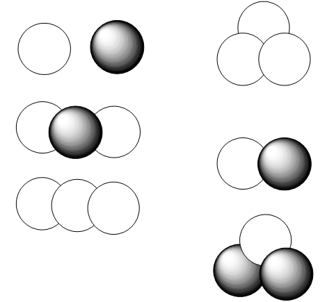
Let’s try another example to practice using Hückel or tight-binding theory. In particular, I’d like you to imagine two possible structures for a cluster of three Na atoms (i.e., pretend that someone came to you and asked what geometry you think such a cluster would assume in its ground electronic state), one linear and one an equilateral triangle. Further, assume that the Na-Na distances in both such clusters are equal (i.e., that the person asking for your theoretical help is willing to assume that variations in bond lengths are not the crucial factor in determining which structure is favored). In Figure 2.11, I shown the two candidate clusters and their 3s orbitals.
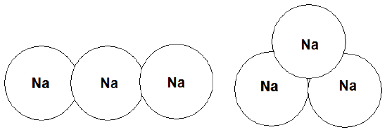
Numbering the three Na atoms’ valence 3s orbitals \(\chi_1\), \(\chi_2\), and \(\chi_3\), we then set up the 3x3 Hückel matrix appropriate to the two candidate structures:
\[
\left[ \begin{array}{ccc}
\alpha & \beta &0\\
\beta & \alpha &\beta\\
0 & \beta & \alpha
\end{array}
\right]
\]
for the linear structure (n.b., the zeros arise because \(\chi_1\) and \(\chi_3\) do not overlap and thus have no \(\beta\) coupling matrix element). Alternatively, for the triangular structure, we find
\[
\left[ \begin{array}{ccc}
\alpha & \beta &\beta\\
\beta & \alpha &\beta\\
\beta & \beta & \alpha
\end{array}
\right]
\]
as the Hückel matrix. Each of these 3x3 matrices will have three eigenvalues that we obtain by subtracting e from their diagonals and setting the determinants of the resulting matrices to zero. For the linear case, doing so generates
\[(\alpha-\varepsilon)^3 – 2 \beta^2 (\alpha-\varepsilon\alpha-\varepsilon) = 0,\]
and for the triangle case it produces
\[(\alpha-\varepsilon)^3 –3 \beta^2 (\alpha-\varepsilon) + 2 \alpha-\varepsilon = 0.\]
The first cubic equation has three solutions that give the MO energies:
\[\varepsilon = \alpha + \sqrt{2} \beta, \varepsilon = \alpha, \text{ and } \varepsilon = \alpha - \sqrt{2} \beta,\]
for the bonding, non-bonding and antibonding MOs, respectively. The second cubic equation also has three solutions
\[\varepsilon = \alpha + 2\beta, \varepsilon = \alpha - \beta , \text{ and } \varepsilon = \alpha - \beta.\]
So, for the linear and triangular structures, the MO energy patterns are as shown in Figure 2.12.

For the neutral \(Na_3\) cluster about which you were asked, you have three valence electrons to distribute among the lowest available orbitals. In the linear case, we place two electrons into the lowest orbital and one into the second orbital. Doing so produces a 3-electron state with a total energy of \(E= 2(\alpha+\sqrt{2} \beta) + \alpha= 3\alpha +2\sqrt{2}\beta\). Alternatively, for the triangular species, we put two electrons into the lowest MO and one into either of the degenerate MOs resulting in a 3-electron state with total energy \(E = 3 \alpha + 3\beta\). Because b is a negative quantity, the total energy of the triangular structure is lower than that of the linear structure since \(3 > 2\sqrt{2}\).
The above example illustrates how we can use Hückel or tight-binding theory to make qualitative predictions (e.g., which of two shapes is likely to be of lower energy).
Notice that all one needs to know to apply such a model to any set of atomic orbitals that overlap to form MOs is
- the individual AO energies a (which relate to the electronegativity of the AOs),
- the degree to which the AOs couple (the b parameters which relate to AO overlaps),
- an assumed geometrical structure whose energy one wants to estimate.
This example and the earlier example pertinent to \(H_2\) or the \(\pi\) bond in ethylene also introduce the idea of symmetry. Knowing, for example, that \(H_2\), ethylene, and linear \(Na_3\) have a left-right plane of symmetry allows us to solve the Hückel problem in terms of symmetry-adapted atomic orbitals rather than in terms of primitive atomic orbitals as we did earlier. For example, for linear \(Na_3\), we could use the following symmetry-adapted functions:
\[\chi_2 {\rm and} \frac{1}{\sqrt{2}} (\chi_1 + \chi_3)\]
both of which are even under reflection through the symmetry plane and
\[ \frac{1}{\sqrt{2}} (\chi_1 - \chi_3)\]
which is odd under reflection. The 3x3 Hückel matrix would then have the form
\[
\left[ \begin{array}{ccc}
\alpha & \sqrt{2}\beta &0\\
\sqrt{2}\beta & \alpha &0\\
0 & 0 & \alpha
\end{array}
\right]
\]
For example, \(H_{1,2}\) and \(H_{2,3}\) are evaluated as follows
\[ H_{1,2} = \langle \frac{1}{\sqrt{2}} (\chi_1 + \chi_3)|H|\chi_2\rangle = 2\frac{1}{\sqrt{2}} \beta\]
\[H_{2,3} = \langle \frac{1}{\sqrt{2}} (\chi_1 + \chi_3)|H| \frac{1}{\sqrt{2}} (\chi_1 - \chi_3)\rangle = \frac{1}{2}( \alpha + \beta - \beta - \alpha)= 0.\]
The three eigenvalues of the above Hückel matrix are easily seen to be \(\alpha\), \(\alpha+\sqrt{2}\beta\), and \(\alpha-\sqrt{2}\beta\), exactly as we found earlier. So, it is not necessary to go through the process of forming symmetry-adapted functions; the primitive Hückel matrix will give the correct answers even if you do not. However, using symmetry allows us to break the full (3x3 in this case) Hückel problem into separate Hückel problems for each symmetry component (one odd function and two even functions in this case, so a 1x1 and a \(2\times2\) sub - matrix).
While we are discussing the issue of symmetry, let me briefly explain the concept of approximate symmetry again using the above Hückel problem as it applies to ethylene as an illustrative example.
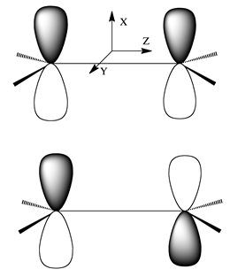
Clearly, as illustrated in Figure 2.12a, at its equilibrium geometry the ethylene molecule has a plane of symmetry (denoted \(\sigma_{X,Y}\)) that maps nuclei and electrons from its left to its right and vice versa. This is the symmetry element that could used to decompose the \(2\times2\) Hückel matrix describing the \(\pi\) and \(\pi^*\) orbitals into two 1x1 matrices. However, if any of the four C-H bond lengths or HCH angles is displaced from its equilibrium value in a manner that destroys the perfect symmetry of this molecule, or if one of the C-H units were replaced by a C-CH3 unit, it might appear that symmetry would no longer be a useful tool in analyzing the properties of this molecule’s molecular orbitals. Fortunately, this is not the case.
Even if there is not perfect symmetry in the nuclear framework of this molecule, the two atomic \(p_\pi\) orbitals will combine to produce a bonding \(\pi\) and antibonding \(\pi^*\) orbital. Moreover, these two molecular orbitals will still possess nodal properties similar to those shown in Figure 2.12a even though they will not possess perfect even and odd character relative to the \(\sigma_{X,Y}\) plane. The bonding orbital will still have the same sign to the left of the \(\sigma_{X,Y}\) plane as it does to the right, and the antibonding orbital will have the opposite sign to the left as it does to the right, but the magnitudes of these two orbitals will not be left-right equal. This is an example of the concept of approximate symmetry. It shows that one can use symmetry, even when it is not perfect, to predict the nodal patterns of molecular orbitals, and it is the nodal patterns that govern the relative energies of orbitals as we have seen time and again.
Let’s see if you can do some of this on your own. Using the above results, would you expect the cation \(Na_3^+\) to be linear or triangular? What about the anion \(Na_3^-\)? Next, I want you to substitute the MO energies back into the 3x3 matrix and find the \(\chi_1\), \(\chi_2\), and \(\chi_3\) coefficients appropriate to each of the 3 MOs of the linear and of the triangular structure. See if doing so leads you to solutions that can be depicted as shown in Figure 2.13, and see if you can place each set of MOs in the proper energy ordering.
Now, I want to show you how to broaden your horizons and use tight-binding theory to describe all of the bonds in a more complicated molecule such as ethylene shown in Figure 2.14. What is different about this kind of molecule when compared with metallic or conjugated species is that the bonding can be described in terms of several pairs of valence orbitals that couple to form two-center bonding and antibonding molecular orbitals. Within the Hückel model described above, each pair of orbitals that touch or overlap gives rise to a 2x2 matrix. More correctly, all n of the constituent valence orbitals form an nxn matrix, but this matrix is broken up into 2x2 blocks. Notice that this did not happen in the triangular Na3 case where each AO touched two other AOs. For the ethlyene case, the valence orbitals consist of (a) four equivalent C \(sp^2\) orbitals that are directed toward the four H atoms, (b) four H \(1s\) orbitals, (c) two C \(sp^2\) orbitals directed toward one another to form the C-C \(\sigma\) bond, and (d) two C \(p_\pi\) orbitals that will form the C-C \(\pi\) bond. This total of 12 orbitals generates 6 Hückel matrices as shown below the ethylene molecule.
We obtain one \(2\times2\) matrix for the C-C \(\sigma\) bond of the form
\[
\left[ \begin{array}{cc}
\alpha_{sp^2} & \beta_{sp^2,sp^2} \\
\beta_{sp^2,sp^2} & \alpha_{sp^2}
\end{array}
\right]
\]
and one \(2\times2\) matrix for the C-C \(\pi\) bond of the form
\[
\left[ \begin{array}{cc}
\alpha_{p_\pi} & \beta_{p_\pi,p_\pi} \\
\beta_{p_\pi,p_\pi} & \alpha_{p_\pi}
\end{array}
\right]
\]
Finally, we also obtain four identical \(2\times2\) matrices for the C-H bonds:
\[
\left[ \begin{array}{cc}
\alpha_{sp^2} & \beta_{sp^2,H} \\
\beta_{sp^2,H} & \alpha_{H}
\end{array}
\right]
\]
The above matrices produce
- four identical C-H bonding MOs having energies \[\varepsilon = \dfrac{(\alpha_H + \alpha_C) –\sqrt{(\alpha_H - \alpha_C)^2 + 2\beta^2}}{2},\]
- four identical C-H antibonding MOs having energies \[\varepsilon^* = \dfrac{(\alpha_H + \alpha_C) + \sqrt{(\alpha_H - \alpha_C)^2 + 2\beta^2}}{2},\]
- one bonding C-C \(\pi\) orbital with \[\varepsilon = \alpha_{p\pi}+ \beta,\]
- a partner antibonding C-C orbital with \[\varepsilon^* = \alpha_{p\pi} - \beta,\]
- a C-C \(\sigma\) bonding MO with \[\varepsilon = \alpha_{sp^2}+ \beta,\] and (\phi) its antibonding partner with \[\varepsilon^* = \alpha_{sp^2}- \beta.\]
In all of these expressions, the \(\beta\) parameter is supposed to be that appropriate to the specific orbitals that overlap as shown in the matrices.
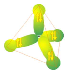
If you wish to practice this exercise of breaking a large molecule down into sets of interacting valence, try to see what Hückel matrices you obtain and what bonding and antibonding MO energies you obtain for the valence orbitals of methane shown in Figure 2.15.
Before leaving this discussion of the Hückel/tight-binding model, I need to stress that it has its flaws (because it is based on approximations and involves neglecting certain terms in the Schrödinger equation). For example, it predicts (see above) that ethylene has four energetically identical C-H bonding MOs (and four degenerate C-H antibonding MOs). However, this is not what is seen when photoelectron spectra are used to probe the energies of these MOs. Likewise, it suggests that methane has four equivalent C-H bonding and antibonding orbitals, which, again is not true. It turns out that, in each of these two cases (ethylene and methane), the experiments indicate a grouping of four nearly iso-energetic bonding MOs and four nearly iso-energetic antibonding MOs. However, there is some “splitting” among these clusters of four MOs. The splittings can be interpreted, within the Hückel model, as arising from couplings or interactions among, for example, one sp2 or \(sp^3\) orbital on a given C atom and another such orbital on the same atom. Such couplings cause the nxn Hückel matrix to not block-partition into groups of \(2\times2\) sub - matrices because now there exist off-diagonal b factors that couple one pair of directed valence to another. When such couplings are included in the analysis, one finds that the clusters of MOs expected to be degenerate are not but are split just as the photoelectron data suggest.
Contributors and Attributions
Jack Simons (Henry Eyring Scientist and Professor of Chemistry, U. Utah) Telluride Schools on Theoretical Chemistry
Integrated by Tomoyuki Hayashi (UC Davis)