2.5: Hydrogenic Orbitals

The Hydrogenic atom problem forms the basis of much of our thinking about atomic structure. To solve the corresponding Schrödinger equation requires separation of the \(r\), \(\theta\), and \(\psi\) variables.

The Schrödinger equation for a single particle of mass \(\mu\) moving in a central potential (one that depends only on the radial coordinate \(r\)) can be written as

\[-\frac{\hbar^2}{2\mu}\left(\frac{\partial^2}{\partial x^2}+\frac{\partial^2}{\partial y^2}+\frac{\partial^2}{\partial z^2}\right)\psi+V(\sqrt{x^2+y^2+z^2}\Psi=E\psi\]

or, introducing the short-hand notation \(\nabla^2\):

\[-\frac{\hbar^2}{2\mu}​ \nabla^2 \psi + V \psi = E\psi.\]

This equation is not separable in Cartesian coordinates (\(x,y,z\)) because of the way \(x,y,\) and \(z\) appear together in the square root. However, it is separable in spherical coordinates where it has the form
\[-\frac{\hbar^2}{2\mu r^2} \left(\frac{\partial}{\partial r}\left(r^2\frac{\partial\psi}{\partial r}\right)\right) -\frac{\hbar^2}{2\mu r^2} \frac{1}{\sin\theta}\frac{\partial}{\partial \theta}\left(\sin\theta\frac{\partial \psi}{\partial\theta}\right) -\frac{\hbar^2}{2\mu r^2}\frac{1}{\sin^2\theta}\frac{\partial^2 \psi}{\partial\theta^2}+V(r)\psi=-\frac{\hbar^2}{2\mu r^2}\nabla^2\Psi+V\psi=E\psi.\]

Subtracting \(V(r) \psi\) from both sides of the equation and multiplying by - then moving the derivatives with respect to \(r\) to the right-hand side, one obtains

\[ \frac{1}{\sin\theta}\frac{\partial}{\partial \theta} \left(\sin\theta\frac{\partial \psi}{\partial\theta} \right) + \frac{1}{\sin^2\theta}\frac{\partial^2 \psi}{\partial\phi^2}
= -\frac{2\mu r^2}{\hbar^2}(E-V(r)) \psi - \left(\frac{\partial}{\partial r}\left(r^2\frac{\partial\psi}{\partial r}\right)\right).\]

Notice that, except for \(\psi\) itself, the right-hand side of this equation is a function of \(r\) only; it contains no \(\theta\) or \(\phi\) dependence. Let's call the entire right hand side \(\Phi(r) \psi\) to emphasize this fact.

To further separate the \(\theta\) and \(\phi\) dependence, we multiply by \(\sin^2\theta\) and subtract the \(\theta\) derivative terms from both sides to obtain

\[\frac{\partial^2 \psi}{\partial\phi^2}= \Phi(r)\psi\sin^2\theta - \sin\theta\frac{\partial}{\partial\theta} \left(\sin\theta\frac{\partial \psi}{\partial\theta} \right).\]

Now we have separated the \(\phi\) dependence from the \(\theta\) and r dependence. We now introduce the procedure used to separate variables in differential equations and assume y can be written as a function of \(\phi\) times a function of \(r\) and \(\theta\): \(\psi = \Phi(\phi) Q(r,\theta)\). Dividing by \(\Phi Q\), we obtain

\[ \frac{1}{\Phi}\frac{\partial^2\Phi}{\partial \phi^2}= \frac{1}{Q}\left(F(r)\sin^2\theta Q-\sin\theta\frac{\partial }{\partial\theta}\left(\sin\theta\frac{\partial Q}{\partial\theta}\right)\right).\]

Now all of the \(\phi\) dependence is isolated on the left hand side; the right hand side contains only \(r\) and \(\theta\) dependence.

Whenever one has isolated the entire dependence on one variable as we have done above for the \(\phi\) dependence, one can easily see that the left and right hand sides of the equation must equal a constant. For the above example, the left hand side contains no \(r\) or \(\theta\) dependence and the right hand side contains no \(\phi\) dependence. Because the two sides are equal for all values of \(r\), \(\theta\), and \(\phi\), they both must actually be independent of \(r\), \(\theta\), and \(\phi\) dependence; that is, they are constant. This again is what is done when one employs the separations of variables method in partial differential equations.

For the above example, we therefore can set both sides equal to a so-called separation constant that we call \(-m^2\). It will become clear shortly why we have chosen to express the constant in the form of minus the square of an integer. You may recall that we studied this same \(\phi\) - equation earlier and learned how the integer \(m\) arises via. the boundary condition that \(\phi\) and \(\phi +2\pi\) represent identical geometries.

The \(\Phi\) Equation

The resulting \(\Phi\) equation reads (the “ symbol is used to represent second derivative)

\[\Phi'' + m^2\Phi = 0.\]

This equation should be familiar because it is the equation that we treated much earlier when we discussed z-component of angular momentum. So, its further analysis should also be familiar, but for completeness, I repeat much of it. The above equation has as its most general solution

\[ \Phi = A e^{im\phi} + B e^{-im\phi} .\]

Because the wave functions of quantum mechanics represent probability densities, they must be continuous and single-valued. The latter condition, applied to our \(\Phi\) function, means (n.b., we used this in our earlier discussion of z-component of angular momentum) that

\[\Phi(\phi) = \Phi(2\pi+\phi) \]

or

\[Ae^{im\phi}(1-e^{2im\pi})+ Be^{-im\phi}(1-e^{2im\pi})​= 0.\]

This condition is satisfied only when the separation constant is equal to an integer \(m = 0, ±1, ± 2, \cdots \). This provides another example of the rule that quantization comes from the boundary conditions on the wave function. Here \(m\) is restricted to certain discrete values because the wave function must be such that when you rotate through \(2\pi\) about the z-axis, you must get back what you started with.

The \(\Theta\) Equation

Now returning to the equation in which the \(\phi\) dependence was isolated from the \(r\) and \(\theta\) dependence and rearranging the \(\theta\) terms to the left-hand side, we have

\[ \frac{1}{\sin\theta}\frac{\partial }{\partial \theta} \left(\sin\theta\frac{\partial Q}{\partial\theta} \right) - \frac{m^2Q}{\sin^2\theta} = F(r)Q.\]

In this equation we have separated the \(\theta\) and \(r\) terms, so we can further decompose the wave function by introducing \(Q = \Theta(\theta) R(r)\), which yields

\[\frac{1}{\Theta\sin\theta}\frac{\partial }{\partial \theta} \left(\sin\theta\frac{\partial \Theta}{\partial\theta} \right) - \frac{m^2}{\sin^2\theta} = \frac{F(r)Q}{R}=-\lambda.\]

where a second separation constant, \(-\lambda\), has been introduced once the \(r\) and \(\theta\) dependent terms have been separated onto the right and left hand sides, respectively.
We now can write the \(\theta\) equation as
\[ \frac{1}{\sin\theta}\frac{\partial }{\partial \theta} \left(\sin\theta\frac{\partial \Theta}{\partial\theta} \right) - \frac{m^2\Theta}{\sin^2\theta} = -\lambda\Theta.\]
where \(m\) is the integer introduced earlier. To solve this equation for \(\Theta\), we make the substitutions \(z =\cos\theta\) and \(P(z) = \Theta(\theta)\), so \(\sqrt{1-z^2}=\sin\theta\), and
\[ \frac{\partial }{\partial \theta} = \frac{\partial z}{\partial \theta}\frac{\partial }{\partial z}= - \sin\theta ​\frac{\partial }{\partial z}.\]

The range of values for \(\theta\) was \(0 \le \theta < \pi\), so the range for \(z\) is \(-1 < z < 1\). The equation for \(\Theta\), when expressed in terms of \(P\) and \(z\), becomes

\[ \frac{d}{dz}\left((1-z^2)\frac{dP}{dz}\right)- \frac{m^2P}{1-z^2}+ \lambda P= 0.\]

Now we can look for polynomial solutions for \(P\), because \(z\) is restricted to be less than unity in magnitude. If \(m\) = 0, we first let

\[ P= \sum_{k=0}a_kz^k,\]

and substitute into the differential equation to obtain

\[ \sum_{k=0}(k+2)(k+1)a_{k+2}z^k - \sum_{k=0}(k+1)ka_{k}z^k+ \lambda\sum_{k=0}a_kz^k = 0.\]

Equating like powers of \(z\) gives

\[ a_{k+2} = \frac{a_k(k(k+1)-\lambda)}{(k+2)(k+1)}.\]

Note that for large values of \(k\)

\[\frac{a_{k+2}}{a_{k}} \rightarrow \frac{k^2\left(1+\frac{1}{k}\right)}{k^2\left(1+\frac{2}{k}\right)\left(1+\frac{1}{k}\right)} = 1.\]

Since the coefficients do not decrease with \(k\) for large \(k\), this series will diverge for \(z = ± 1\) unless it truncates at finite order. This truncation only happens if the separation constant \(\lambda\) obeys \(\lambda = \lambda(\lambda+1)\), where \(l\) is an integer (you can see this from the recursion relation giving \(a_{k+2}\) in terms of \(a_k\); only for certain values of \(l\) will the numerator vanish ). So, once again, we see that a boundary condition (i.e., that the wave function not diverge and thus be normalizable in this case) give rise to quantization. In this case, the values of \(l\) are restricted to \(\lambda(\lambda+1)\); before, we saw that \(m\) is restricted to \(0, ±1, ± 2, \cdots \).
Since the above recursion relation links every other coefficient, we can choose to solve for the even and odd functions separately. Choosing \(a_0\) and then determining all of the even \(a_k\)​ in terms of this \(a_1\)​, followed by rescaling all of these \(a_k\)​ to make the function normalized generates an even solution. Choosing \(a_1\)​ and determining all of the odd \(a_k\)​ in like manner, generates an odd solution.
For \(l= 0\), the series truncates after one term and results in \(P_o(z) = 1\). For \(l= 1\) the same thing applies and \(P_1(z) = z\). For \(l= 2\), \(a_2 = -6 \dfrac{a_o}{2}= -3a_o\), so one obtains \(P_2 = 3z^2-1\), and so on. These polynomials are called Legendre polynomials and are denoted \(P_l(z)\).
For the more general case where \(m \ne 0\), one can proceed as above to generate a polynomial solution for the \(Q\) function. Doing so, results in the following solutions:
\[P_l^m(z)=(1-z^2)^{|m|/2}\frac{d^{|m|}P_l(z)}{dz^{|m|}}\]
These functions are called Associated Legendre polynomials, and they constitute the solutions to the \(Q\) problem for non-zero \(m\) values.
The above \(P\) and \(e^{im\phi}\) functions, when re-expressed in terms of \(\theta\) and \(\phi\), yield the full angular part of the wave function for any centrosymmetric potential. These solutions are usually written as

\[Y_{l,m}(\theta,\phi)= P_l^m(\cos\theta)\frac{1}{\sqrt{2\pi}} \exp(im\phi),\]

and are called spherical harmonics. They provide the angular solution of the \(r,\theta,\phi\) Schrödinger equation for any problem in which the potential depends only on the radial coordinate. Such situations include all one-electron atoms and ions (e.g., \(H\), \(He^+\), \(Li^{2+}\), etc.), the rotational motion of a diatomic molecule (where the potential depends only on bond length \(r\)), the motion of a nucleon in a spherically symmetrical box (as occurs in the shell model of nuclei), and the scattering of two atoms (where the potential depends only on interatomic distance).
The \(Y_{l,m}\) functions possess varying number of angular nodes, which, as noted earlier, give clear signatures of the angular or rotational energy content of the wave function. These angular nodes originate in the oscillatory nature of the Legendre and associated Legendre polynomials \(P_{lm}(\cos\theta)\); the higher \(l\) is, the more sign changes occur within the polynomial.

The \(R\) Equation

Let us now turn our attention to the radial equation, which is the only place that the explicit form of the potential appears. Using our earlier results for the equation obeyed by the \(R(r)\) function and specifying \(V(r)\) to be the Coulomb potential appropriate for an electron in the field of a nucleus of charge \(+Z_e\), yields:

\[\frac{1}{r^2}\frac{d}{dr}\left(r^2\frac{dR}{dr}\right)+\left(\frac{2\mu}{\hbar^2}\left(E+\frac{Ze^2}{r}\right)-\frac{L(L+1)}{rZ2}\right) R = 0.\]

We can simplify things considerably if we choose rescaled length and energy units because doing so removes the factors that depend on \(\mu\), \(\hbar\), and \(e\). We introduce a new radial coordinate \(\rho\) and \(a\) quantity \(\sigma\) as follows:

\[\rho=r\sqrt{\frac{-8\mu E}{\hbar^2}} \text{ and } \sigma = \frac{\mu Ze^2}{\hbar\sqrt{-2\mu E}}.\]

Notice that if \(E\) is negative, as it will be for bound states (i.e., those states with energy below that of a free electron infinitely far from the nucleus and with zero kinetic energy), \(\rho\) and \(\sigma\) are real. On the other hand, if \(E\) is positive, as it will be for states that lie in the continuum, \(\rho\) and \(\sigma\) will be imaginary. These two cases will give rise to qualitatively different behavior in the solutions of the radial equation developed below.

We now define a function \(S\) such that \(S(\rho) = R(r)\) and substitute \(S\) for \(R\) to obtain:

\[\frac{1}{\rho^2}\frac{d}{d\rho}\left(\rho^2\frac{dS}{d\rho}\right) + \left(-\frac{1}{4}-\frac{L(L+1)}{\rho^2}+\dfrac{\sigma}{\rho}\right) S = 0.\]

The differential operator terms can be recast in several ways using

\[\frac{1}{\rho^2}\frac{d}{d\rho}\left(\rho^2\frac{dS}{d\rho}\right)=\frac{d^2 S}{d\rho^2} +\frac{2}{\rho}\frac{dS}{d\rho} =\frac{1}{\rho}\frac{d^2}{d\rho^2}(\rho S) .\]

The strategy that we now follow is characteristic of solving second order differential equations. We will examine the equation for \(S\) at large and small \(\rho\) values. Having found solutions at these limits, we will use a power series in \(\rho\) to interpolate between these two limits.

Let us begin by examining the solution of the above equation at small values of \(\rho\) to see how the radial functions behave at small \(\rho\). As \(\rho\rightarrow0\), the term \(-\dfrac{L(L+1)}{\rho^2}\) will dominate over \(-\dfrac{1}{4} +\dfrac{\sigma}{\rho}\). Neglecting these other two terms, we find that, for small values of \(\rho\) (or \(r\)), the solution should behave like \(\rho^L\) and because the function must be normalizable, we must have \(L \ge 0\). Since \(l\) can be any non-negative integer, this suggests the following more general form for \(S(r)\):
\[ S(\rho) \approx \rho^L e^{-a\rho}.\]
This form will insure that the function is normalizable since \(S(r) \rightarrow 0\) as \(r \rightarrow \infty\) for all \(L\), as long as \(\rho\) is a real quantity. If \(\rho\) is imaginary, such a form may not be normalized (see below for further consequences).
Turning now to the behavior of \(S\) for large \(\rho\), we make the substitution of \(S(r)\) into the above equation and keep only the terms with the largest power of \(\rho\) (i.e., the \(-1/4\) term) and we allow the derivatives in the above differential equation to act on \(\approx \rho^L e^{-a\rho}​\). Upon so doing, we obtain the equation
\[ a^2\rho^Le^{-a\rho} = \frac{1}{4}\rho^Le^{-a\rho}​ ,\]
which leads us to conclude that the exponent in the large-\(r\) behavior of S is \(a = \dfrac{1}{2}\).
Having found the small-\(\rho\) and large-\(\rho\) behaviors of \(S(\rho)\), we can take \(S\) to have the following form to interpolate between large and small r-values:
\[S(\rho) = \rho^L​e^{-\frac{\rho}{2}}​​P(\rho),\]
where the function \(P\) is expanded in an infinite power series in \(\rho\) as \(P(\rho) =\sum a_k\rho^k\). Again substituting this expression for \(S\) into the above equation we obtain
\[P"\rho + P'(2L+2-\rho) + P(\sigma-L-l) = 0,\]
and then substituting the power series expansion of \(P\) and solving for the ak's we arrive at a recursion relation for the ak coefficients:
\[a_{k+1} = \frac{(k-\sigma+L+1)a_k}{(k+1)(k+2L+2)}.\]
For large \(k\), the ratio of expansion coefficients reaches the limit \(\dfrac{a_{k+1}}{a_k}=\dfrac{1}{k}\), which, when substituted into \(\sum a_k\rho^k\), gives the same behavior as the power series expansion of \(e^\rho\). Because the power series expansion of \(P\) describes a function that behaves like \(e^\rho\)​ for large \(\rho\), the resulting \(S(\rho)\) function would not be normalizable because the efactor would be overwhelmed by this \(e^\rho\) dependence. Hence, the series expansion of \(P\) must truncate in order to achieve a normalizable \(S\) function. Notice that if \(\rho\) is imaginary, as it will be if \(E\) is in the continuum, the argument that the series must truncate to avoid an exponentially diverging function no longer applies. Thus, we see a key difference between bound (with \(\rho\) real) and continuum (with r imaginary) states. In the former case, the boundary condition of non-divergence arises; in the latter, it does not because \(e^{\frac{\rho}{2}}\) does not diverge if \(\rho\) is imaginary.

To truncate at a polynomial of order \(n'\), we must have \(n'-s+L+l= 0\). This implies that the quantity s introduced previously is restricted to \(s = n'+L+l\), which is certainly an integer; let us call this integer \(n\). If we label states in order of increasing \(n = 1,2,3,\cdots \), we see that doing so is consistent with specifying a maximum order (\(n'\)) in the \(P(r)\) polynomial \(n' = 0,1,2,\cdots \) after which the \(\textbf{L}_{-}\) value can run from \(L = 0\), in steps of unity up to \(L = n-1\).

Substituting the integer \(n\) for \(s\), we find that the energy levels are quantized because \(s\) is quantized (equal to \(n\)):

\[E = -\frac{\mu Z^2 e^4}{2\hbar^2 n^2}\]

and the scaled distance turns out to be

\[\rho = \frac{Zr}{a_0n}.\]​

Here, the length \(a_o=\dfrac{\hbar^2}{\mu e^2}\) is the so-called Bohr radius , which turns out to be 0.529 Å; it appears once the above E-expression is substituted into the equation for \(\rho\). Using the recursion equation to solve for the polynomial's coefficients \(a_k\) for any choice of \(n\) and \(L\) quantum numbers generates a so-called Laguerre polynomial; \(P_{n-L-1}(\rho)\). They contain powers of \(\rho\) from zero through \(n-L-1\), and they have \(n-L-1\) sign changes as the radial coordinate ranges from zero to infinity. It is these sign changes in the Laguerre polynomials that cause the radial parts of the hydrogenic wave functions to have \(n-L-1\) nodes. For example, \(3d\) orbitals have no radial nodes, but 4d orbitals have one; and, as shown in Figure 2.16, \(3p\) orbitals have one while \(3s\) orbitals have two. Once again, the higher the number of nodes, the higher the energy in the radial direction.

Figure 2.16. Plots of the probability densities \(r^2|R(r)|^2\) of the radial parts of the \(3s\) and \(3p\) orbitals

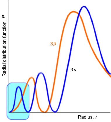
Let me again remind you about the danger of trying to understand quantum wave functions or probabilities in terms of classical dynamics. What kind of potential \(V(r)\) would give rise to, for example, the \(3s\) \(P(r)\) plot shown above? Classical mechanics suggests that \(P\) should be large where the particle moves slowly and small where it moves quickly. So, the \(3s\) \(P(r)\) plot suggests that the radial speed of the electron has three regions where it is low (i.e., where the peaks in \(P\) are) and two regions where it is very large (i.e., where the nodes are). This, in turn, suggests that the radial potential \(V(r)\) experienced by the \(3s\) electron is high in three regions (near peaks in P) and low in two regions. Of course, this conclusion about the form of \(V(r)\) is nonsense and again illustrates how one must not be drawn into trying to think of the classical motion of the particle, especially for quantum states with small quantum number. In fact, the low quantum number states of such one-electron atoms and ions have their radial \(P(r)\) plots focused in regions of r-space where the potential \(–Ze^2/r\) is most attractive (i.e., largest in magnitude).

Finally, we note that the energy quantization does not arise for states lying in the continuum because the condition that the expansion of \(P(r)\) terminate does not arise. The solutions of the radial equation appropriate to these scattering states (which relate to the scattering motion of an electron in the field of a nucleus of charge \(Z\)) are a bit outside the scope of this text, so we will not treat them further here.

To review, separation of variables has been used to solve the full \(r,\theta,\phi\) Schrödinger equation for one electron moving about a nucleus of charge \(Z\). The \(\theta\) and \(\phi\) solutions are the spherical harmonics \(Y_{L,m} (\theta,\phi)\). The bound-state radial solutions

\[R_{n,L}(r) = S(\rho) = \rho^Le^{-\frac{\rho}{2}}P_{n-L-1}(\rho)\]

depend on the \(n\) and \(L\) quantum numbers and are given in terms of the Laguerre polynomials.

Summary

To summarize, the quantum numbers \(L\) and \(m\) arise through boundary conditions requiring that \(\psi(\theta)\) be normalizable (i.e., not diverge) and \(\psi(\phi) = \psi(\phi+2\pi)\). The radial equation, which is the only place the potential energy enters, is found to possess both bound-states (i.e., states whose energies lie below the asymptote at which the potential vanishes and the kinetic energy is zero) and continuum states lying energetically above this asymptote. The former states are spatially confined by the potential, but the latter are not. The resulting hydrogenic wave functions (angular and radial) and energies are summarized on pp. 133-136 in the text by L. Pauling and E. B. Wilson for \(n\) up to and including 6 and \(L\) up to 5 (i.e, for \(s, p, d, f, g,\) and \(h\) orbitals).

There are both bound and continuum solutions to the radial Schrödinger equation for the attractive coulomb potential because, at energies below the asymptote, the potential confines the particle between \(r=0\) and an outer classical turning point, whereas at energies above the asymptote, the particle is no longer confined by an outer turning point (see Figure 2.17). This provides yet another example of how quantized states arise when the potential spatially confines the particle, but continuum states arise when the particle is not spatially confined.

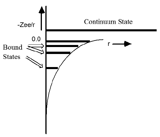
Figure 2.17: Radial Potential for Hydrogenic Atoms and Bound and Continuum Orbital Energies.

The solutions of this one-electron problem form the qualitative basis for much of atomic and molecular orbital theory. For this reason, the reader is encouraged to gain a firmer understanding of the nature of the radial and angular parts of these wave functions. The orbitals that result are labeled by \(n\), \(l\), and \(m\) quantum numbers for the bound states and by \(l\) and \(m\) quantum numbers and the energy \(E\) for the continuum states. Much as the particle-in-a-box orbitals are used to qualitatively describe p- electrons in conjugated polyenes, these so-called hydrogen-like orbitals provide qualitative descriptions of orbitals of atoms with more than a single electron. By introducing the concept of screening as a way to represent the repulsive interactions among the electrons of an atom, an effective nuclear charge \(Z_{\rm eff}\) can be used in place of \(Z\) in the \(\psi_{n,l,m}\) and \(E_n\) to generate approximate atomic orbitals to be filled by electrons in a many-electron atom. For example, in the crudest approximation of a carbon atom, the two \(1s\) electrons experience the full nuclear attraction so \(Z_{\rm eff} = 6\) for them, whereas the \(2s\) and \(2p\) electrons are screened by the two \(1s\) electrons, so \(Z_{\rm eff} = 4\) for them. Within this approximation, one then occupies two \(1s\) orbitals with \(Z = 6\), two \(2s\) orbitals with \(Z = 4\) and two \(2p\) orbitals with \(Z=4\) in forming the full six-electron wave function of the lowest-energy state of carbon. It should be noted that the use of screened nuclear charges as just discussed is different from the use of a quantum defect parameter d as discussed regarding Rydberg orbitals in Chapter 1. The \(Z = 4\) screened charge for carbon’s \(2s\) and \(2p\) orbitals is attempting to represent the effect of the inner-shell \(1s\) electrons on the \(2s\) and \(2p\) orbitals. The modification of the principal quantum number made by replacing \(n\) by \((n- d)\) represents the penetration of the orbital with nominal quantum number \(n\) inside its inner-shells.

Contributors and Attributions

Jack Simons (Henry Eyring Scientist and Professor of Chemistry, U. Utah) Telluride Schools on Theoretical Chemistry

Integrated by Tomoyuki Hayashi (UC Davis)