2.3: Densities of States in 1, 2, and 3 dimensions
- Page ID
- 11574
\( \newcommand{\vecs}[1]{\overset { \scriptstyle \rightharpoonup} {\mathbf{#1}} } \)
\( \newcommand{\vecd}[1]{\overset{-\!-\!\rightharpoonup}{\vphantom{a}\smash {#1}}} \)
\( \newcommand{\dsum}{\displaystyle\sum\limits} \)
\( \newcommand{\dint}{\displaystyle\int\limits} \)
\( \newcommand{\dlim}{\displaystyle\lim\limits} \)
\( \newcommand{\id}{\mathrm{id}}\) \( \newcommand{\Span}{\mathrm{span}}\)
( \newcommand{\kernel}{\mathrm{null}\,}\) \( \newcommand{\range}{\mathrm{range}\,}\)
\( \newcommand{\RealPart}{\mathrm{Re}}\) \( \newcommand{\ImaginaryPart}{\mathrm{Im}}\)
\( \newcommand{\Argument}{\mathrm{Arg}}\) \( \newcommand{\norm}[1]{\| #1 \|}\)
\( \newcommand{\inner}[2]{\langle #1, #2 \rangle}\)
\( \newcommand{\Span}{\mathrm{span}}\)
\( \newcommand{\id}{\mathrm{id}}\)
\( \newcommand{\Span}{\mathrm{span}}\)
\( \newcommand{\kernel}{\mathrm{null}\,}\)
\( \newcommand{\range}{\mathrm{range}\,}\)
\( \newcommand{\RealPart}{\mathrm{Re}}\)
\( \newcommand{\ImaginaryPart}{\mathrm{Im}}\)
\( \newcommand{\Argument}{\mathrm{Arg}}\)
\( \newcommand{\norm}[1]{\| #1 \|}\)
\( \newcommand{\inner}[2]{\langle #1, #2 \rangle}\)
\( \newcommand{\Span}{\mathrm{span}}\) \( \newcommand{\AA}{\unicode[.8,0]{x212B}}\)
\( \newcommand{\vectorA}[1]{\vec{#1}} % arrow\)
\( \newcommand{\vectorAt}[1]{\vec{\text{#1}}} % arrow\)
\( \newcommand{\vectorB}[1]{\overset { \scriptstyle \rightharpoonup} {\mathbf{#1}} } \)
\( \newcommand{\vectorC}[1]{\textbf{#1}} \)
\( \newcommand{\vectorD}[1]{\overrightarrow{#1}} \)
\( \newcommand{\vectorDt}[1]{\overrightarrow{\text{#1}}} \)
\( \newcommand{\vectE}[1]{\overset{-\!-\!\rightharpoonup}{\vphantom{a}\smash{\mathbf {#1}}}} \)
\( \newcommand{\vecs}[1]{\overset { \scriptstyle \rightharpoonup} {\mathbf{#1}} } \)
\( \newcommand{\vecd}[1]{\overset{-\!-\!\rightharpoonup}{\vphantom{a}\smash {#1}}} \)
\(\newcommand{\avec}{\mathbf a}\) \(\newcommand{\bvec}{\mathbf b}\) \(\newcommand{\cvec}{\mathbf c}\) \(\newcommand{\dvec}{\mathbf d}\) \(\newcommand{\dtil}{\widetilde{\mathbf d}}\) \(\newcommand{\evec}{\mathbf e}\) \(\newcommand{\fvec}{\mathbf f}\) \(\newcommand{\nvec}{\mathbf n}\) \(\newcommand{\pvec}{\mathbf p}\) \(\newcommand{\qvec}{\mathbf q}\) \(\newcommand{\svec}{\mathbf s}\) \(\newcommand{\tvec}{\mathbf t}\) \(\newcommand{\uvec}{\mathbf u}\) \(\newcommand{\vvec}{\mathbf v}\) \(\newcommand{\wvec}{\mathbf w}\) \(\newcommand{\xvec}{\mathbf x}\) \(\newcommand{\yvec}{\mathbf y}\) \(\newcommand{\zvec}{\mathbf z}\) \(\newcommand{\rvec}{\mathbf r}\) \(\newcommand{\mvec}{\mathbf m}\) \(\newcommand{\zerovec}{\mathbf 0}\) \(\newcommand{\onevec}{\mathbf 1}\) \(\newcommand{\real}{\mathbb R}\) \(\newcommand{\twovec}[2]{\left[\begin{array}{r}#1 \\ #2 \end{array}\right]}\) \(\newcommand{\ctwovec}[2]{\left[\begin{array}{c}#1 \\ #2 \end{array}\right]}\) \(\newcommand{\threevec}[3]{\left[\begin{array}{r}#1 \\ #2 \\ #3 \end{array}\right]}\) \(\newcommand{\cthreevec}[3]{\left[\begin{array}{c}#1 \\ #2 \\ #3 \end{array}\right]}\) \(\newcommand{\fourvec}[4]{\left[\begin{array}{r}#1 \\ #2 \\ #3 \\ #4 \end{array}\right]}\) \(\newcommand{\cfourvec}[4]{\left[\begin{array}{c}#1 \\ #2 \\ #3 \\ #4 \end{array}\right]}\) \(\newcommand{\fivevec}[5]{\left[\begin{array}{r}#1 \\ #2 \\ #3 \\ #4 \\ #5 \\ \end{array}\right]}\) \(\newcommand{\cfivevec}[5]{\left[\begin{array}{c}#1 \\ #2 \\ #3 \\ #4 \\ #5 \\ \end{array}\right]}\) \(\newcommand{\mattwo}[4]{\left[\begin{array}{rr}#1 \amp #2 \\ #3 \amp #4 \\ \end{array}\right]}\) \(\newcommand{\laspan}[1]{\text{Span}\{#1\}}\) \(\newcommand{\bcal}{\cal B}\) \(\newcommand{\ccal}{\cal C}\) \(\newcommand{\scal}{\cal S}\) \(\newcommand{\wcal}{\cal W}\) \(\newcommand{\ecal}{\cal E}\) \(\newcommand{\coords}[2]{\left\{#1\right\}_{#2}}\) \(\newcommand{\gray}[1]{\color{gray}{#1}}\) \(\newcommand{\lgray}[1]{\color{lightgray}{#1}}\) \(\newcommand{\rank}{\operatorname{rank}}\) \(\newcommand{\row}{\text{Row}}\) \(\newcommand{\col}{\text{Col}}\) \(\renewcommand{\row}{\text{Row}}\) \(\newcommand{\nul}{\text{Nul}}\) \(\newcommand{\var}{\text{Var}}\) \(\newcommand{\corr}{\text{corr}}\) \(\newcommand{\len}[1]{\left|#1\right|}\) \(\newcommand{\bbar}{\overline{\bvec}}\) \(\newcommand{\bhat}{\widehat{\bvec}}\) \(\newcommand{\bperp}{\bvec^\perp}\) \(\newcommand{\xhat}{\widehat{\xvec}}\) \(\newcommand{\vhat}{\widehat{\vvec}}\) \(\newcommand{\uhat}{\widehat{\uvec}}\) \(\newcommand{\what}{\widehat{\wvec}}\) \(\newcommand{\Sighat}{\widehat{\Sigma}}\) \(\newcommand{\lt}{<}\) \(\newcommand{\gt}{>}\) \(\newcommand{\amp}{&}\) \(\definecolor{fillinmathshade}{gray}{0.9}\)When a large number of neighboring orbitals overlap, bands are formed. However, the natures of these bands, their energy patterns, and their densities of states are very different in different dimensions.
Before leaving our discussion of bands of orbitals and orbital energies in solids, I want to address a bit more the issue of the density of electronic states and what determines the energy range into which orbitals of a given band will split. First, let’s recall the energy expression for the 1 and 2- dimensional electron in a box case, and let’s generalize it to three dimensions. The general result is
\[E = \sum_j \dfrac{n_j^2 \pi^2\hbar^2}{2mL_j^2}\tag{2.3.1}\]
where the sum over \(j\) runs over the number of dimensions (1, 2, or 3), and \(L_j\) is the length of the box along the jth direction. For one dimension, one observes a pattern of energy levels that grows with increasing \(n\), and whose spacing between neighboring energy levels also grows as a result of which the state density decreases with increasing \(n\). However, in 2 and 3 dimensions, the pattern of energy level spacing displays a qualitatively different character, especially at high quantum number.
Consider first the 3-dimensional case and, for simplicity, let’s use a box that has equal length sides \(L\). In this case, the total energy \(E\) is \(\dfrac{\hbar^2\pi^2}{2mL^2}\) times \((n_x^2 + n_y^2 + n_z^2)\). The latter quantity can be thought of as the square of the length of a vector \(\textbf{R}\) having three components \(n_x\), \(n_y\), \(n_z\). Now think of three Cartesian axes labeled \(n_x\), \(n_y\), and \(n_z\) and view a sphere of radius \(R\) in this space. The volume of the 1/8 th sphere having positive values of \(n_x\), \(n_y\), and \(n_z\) and having radius \(R\) is \(\dfrac{1}{8} \Big(\dfrac{4}{3} \pi R^3\Big)\). Because each cube having unit length along the \(n_x\), \(n_y\), and \(n_z\) axes corresponds to a single quantum wave function and its energy, the total number \(N_{\rm tot}(E)\) of quantum states with positive \(n_x\), \(n_y\), and \(n_z\) and with energy between zero and \(E = \bigg(\dfrac{\hbar^2\pi^2}{2mL^2}\bigg)R^2\) is
\[N_{tot} = \frac{1}{8} (\frac{4}{3} \pi R^3) = \frac{1}{8} \bigg(\frac{4}{3} \pi \left[\frac{2mEL^2}{\hbar^2\pi^2}\right]^{3/2}\bigg)\tag{2.3.2}\]
The number of quantum states with energies between \(E\) and \(E+dE\) is \(\dfrac{dN_{tot}}{dE}dE\), which gives the density \(\Omega(E)\) of states near energy \(E\):
\[\Omega(E) = \frac{dN_{tot}}{dE} = \frac{1}{8} \bigg(\frac{4}{3} \pi \left[\frac{2mEL^2}{\hbar^2\pi^2}\right]^{3/2} \frac{3}{2} \sqrt{E}\bigg). \tag{2.3.3}\]
Notice that this state density increases as \(E\) increases. This means that, in the 3-dimensional case, the number of quantum states per unit energy grows; in other words, the spacing between neighboring state energies decreases, very unlike the 1-dimensioal case where the spacing between neighboring states grows as \(n\) and thus \(E\) grows. This growth in state density in the 3-dimensional case is a result of the degeneracies and near-degeneracies that occur. For example, the states with \(n_x\), \(n_y\), \(n_z\) = 2,1,1 and 1, 1, 2, and 1, 2, 1 are degenerate, and those with \(n_x\), \(n_y\), \(n_z\) = 5, 3, 1 or 5, 1, 3 or 1, 3, 5 or 1, 5, 3 or 3, 1, 5 or 3, 5, 1 are degenerate and nearly degenerate to those having quantum numbers 4, 4, 1 or 1, 4, 4, or 4, 1, 4.
In the 2-dimensional case, degeneracies also occur and cause the density of states to possess an \(E\)-dependence that differs from the 1- or 3-dimensional case. In this situation
, we think of states having energy \(E = \bigg(\dfrac{\hbar^2\pi^2}{2mL^2}\bigg)R^2\), but with \(R^2 = n_x^2 + n_y^2\). The total number of states having energy between zero and \(E\) is
\[N_{\rm total}= 4\pi R^2 = 4\pi E\left(\frac{2mL^2}{\hbar^2\pi^2}\right) \tag{2.3.4}\]
So, the density of states between \(E\) and \(E+dE\) is
\[\Omega(E) = \frac{dN_{\rm total}}{dE} = 4\pi \left(\frac{2mL^2}{\hbar^2\pi^2}\right) \tag{2.3.5}\]
That is, in this 2-dimensional case, the number of states per unit energy is constant for high \(E\) values (where the analysis above applies best).
This kind of analysis for the 1-dimensional case gives
\[N_{\rm total}= R = \sqrt{\frac{2mEL^2}{\hbar^2\pi^2}} \tag{2.3.6}\]
so, the state density between \(E\) and \(E+ dE\) is:
\[\Omega(E) = \frac{1}{2} \sqrt{\frac{2mL^2}{\hbar^2\pi^2}}\frac{1}{2} E^{-1/2}, \tag{2.3.7}\]
which clearly shows the widening spacing, and thus lower state density, as one goes to higher energies.
These findings about densities of states in 1-, 2-, and 3- dimensions are important because, in various problems one encounters in studying electronic states of extended systems such as solids, chains, and surfaces, one needs to know how the number of states available at a given total energy \(E\) varies with \(E\). A similar situation occurs when describing the translational states of an electron or a photo ejected from an atom or molecule into the vacuum; here the 3-dimensional density of states applies. Clearly, the state density depends upon the dimensionality of the problem, and this fact is what I want the students reading this text to keep in mind.
Before closing this Section, it is useful to overview how the various particle-in-box models can be used as qualitative descriptions for various chemical systems.
1a. The one-dimensional box model is most commonly used to model electronic orbitals in delocalized linear polyenes.
1b. The electron-on-a-circle model is used to describe orbitals in a conjugated cyclic ring such as in benzene.
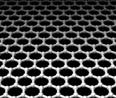
2a. The rectangular box model can be used to model electrons moving within thin layers of metal deposited on a substrate or to model electrons in aromatic sheets such as graphene shown below in Figure 2.8a.

2b. The particle-within-a-circle model can describe states of electrons (or other light particles requiring quantum treatment) constrained within a circular corral.
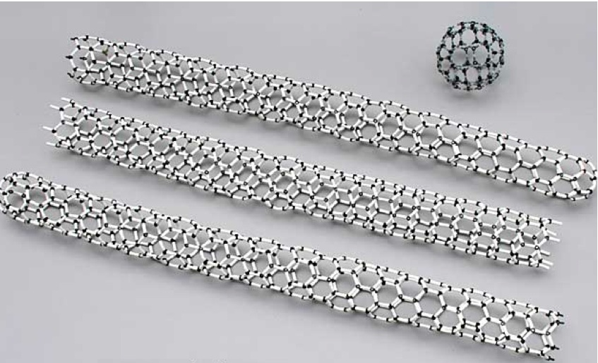
2c. The particle-on-a-sphere’s surface model can describe states of electrons delocalized over the surface of fullerene-type species such as shown in the upper right of Figure 2.8b.

3a. The particle-in-a-sphere model, as discussed earlier, is often used to treat electronic orbitals of quasi-spherical nano-clusters composed of metallic atoms.
3b. The particle-in-a-cube model is often used to describe the bands of electronic orbitals that arise in three-dimensional crystals constructed from metallic atoms.
In all of these models, the potential \(V_0\), which is constant in the region where the electron is confined, controls the energies of all the quantum states relative to that of a free electron (i.e., an electron in vacuum with no kinetic energy).
For some dimensionalities and geometries, it may be necessary to invoke more than one of these models to qualitatively describe the quantum states of systems for which the valence electrons are highly delocalized (e.g., metallic clusters and conjugated organics). For example, for electrons residing on the surface of any of the three graphene tubes shown in Figure 2.8b, one expects quantum states (i) labeled with an angular momentum quantum number and characterizing the electrons’ angular motions about the long axis of the tube, but also (ii) labeled by a long-axis quantum number characterizing the electron’s energy component along the tube’s long axis. For a three-dimensional tube-shaped nanoparticle composed of metallic atoms, one expects the quantum states to be (i) labeled with an angular momentum quantum number and a radial quantum number characterizing the electrons’ angular motions about the long axis of the tube and its radial (Bessel function) character, but again also (ii) labeled by a long-axis quantum number characterizing the electron’s energy component along the tube’s long axis.
Contributors and Attributions
Jack Simons (Henry Eyring Scientist and Professor of Chemistry, U. Utah) Telluride Schools on Theoretical Chemistry
Integrated by Tomoyuki Hayashi (UC Davis)


