6.7: Energy Diagrams
- Page ID
- 30375
\( \newcommand{\vecs}[1]{\overset { \scriptstyle \rightharpoonup} {\mathbf{#1}} } \)
\( \newcommand{\vecd}[1]{\overset{-\!-\!\rightharpoonup}{\vphantom{a}\smash {#1}}} \)
\( \newcommand{\dsum}{\displaystyle\sum\limits} \)
\( \newcommand{\dint}{\displaystyle\int\limits} \)
\( \newcommand{\dlim}{\displaystyle\lim\limits} \)
\( \newcommand{\id}{\mathrm{id}}\) \( \newcommand{\Span}{\mathrm{span}}\)
( \newcommand{\kernel}{\mathrm{null}\,}\) \( \newcommand{\range}{\mathrm{range}\,}\)
\( \newcommand{\RealPart}{\mathrm{Re}}\) \( \newcommand{\ImaginaryPart}{\mathrm{Im}}\)
\( \newcommand{\Argument}{\mathrm{Arg}}\) \( \newcommand{\norm}[1]{\| #1 \|}\)
\( \newcommand{\inner}[2]{\langle #1, #2 \rangle}\)
\( \newcommand{\Span}{\mathrm{span}}\)
\( \newcommand{\id}{\mathrm{id}}\)
\( \newcommand{\Span}{\mathrm{span}}\)
\( \newcommand{\kernel}{\mathrm{null}\,}\)
\( \newcommand{\range}{\mathrm{range}\,}\)
\( \newcommand{\RealPart}{\mathrm{Re}}\)
\( \newcommand{\ImaginaryPart}{\mathrm{Im}}\)
\( \newcommand{\Argument}{\mathrm{Arg}}\)
\( \newcommand{\norm}[1]{\| #1 \|}\)
\( \newcommand{\inner}[2]{\langle #1, #2 \rangle}\)
\( \newcommand{\Span}{\mathrm{span}}\) \( \newcommand{\AA}{\unicode[.8,0]{x212B}}\)
\( \newcommand{\vectorA}[1]{\vec{#1}} % arrow\)
\( \newcommand{\vectorAt}[1]{\vec{\text{#1}}} % arrow\)
\( \newcommand{\vectorB}[1]{\overset { \scriptstyle \rightharpoonup} {\mathbf{#1}} } \)
\( \newcommand{\vectorC}[1]{\textbf{#1}} \)
\( \newcommand{\vectorD}[1]{\overrightarrow{#1}} \)
\( \newcommand{\vectorDt}[1]{\overrightarrow{\text{#1}}} \)
\( \newcommand{\vectE}[1]{\overset{-\!-\!\rightharpoonup}{\vphantom{a}\smash{\mathbf {#1}}}} \)
\( \newcommand{\vecs}[1]{\overset { \scriptstyle \rightharpoonup} {\mathbf{#1}} } \)
\(\newcommand{\longvect}{\overrightarrow}\)
\( \newcommand{\vecd}[1]{\overset{-\!-\!\rightharpoonup}{\vphantom{a}\smash {#1}}} \)
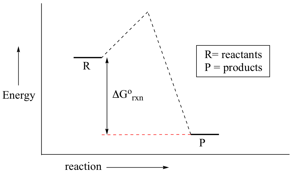
\(\newcommand{\avec}{\mathbf a}\) \(\newcommand{\bvec}{\mathbf b}\) \(\newcommand{\cvec}{\mathbf c}\) \(\newcommand{\dvec}{\mathbf d}\) \(\newcommand{\dtil}{\widetilde{\mathbf d}}\) \(\newcommand{\evec}{\mathbf e}\) \(\newcommand{\fvec}{\mathbf f}\) \(\newcommand{\nvec}{\mathbf n}\) \(\newcommand{\pvec}{\mathbf p}\) \(\newcommand{\qvec}{\mathbf q}\) \(\newcommand{\svec}{\mathbf s}\) \(\newcommand{\tvec}{\mathbf t}\) \(\newcommand{\uvec}{\mathbf u}\) \(\newcommand{\vvec}{\mathbf v}\) \(\newcommand{\wvec}{\mathbf w}\) \(\newcommand{\xvec}{\mathbf x}\) \(\newcommand{\yvec}{\mathbf y}\) \(\newcommand{\zvec}{\mathbf z}\) \(\newcommand{\rvec}{\mathbf r}\) \(\newcommand{\mvec}{\mathbf m}\) \(\newcommand{\zerovec}{\mathbf 0}\) \(\newcommand{\onevec}{\mathbf 1}\) \(\newcommand{\real}{\mathbb R}\) \(\newcommand{\twovec}[2]{\left[\begin{array}{r}#1 \\ #2 \end{array}\right]}\) \(\newcommand{\ctwovec}[2]{\left[\begin{array}{c}#1 \\ #2 \end{array}\right]}\) \(\newcommand{\threevec}[3]{\left[\begin{array}{r}#1 \\ #2 \\ #3 \end{array}\right]}\) \(\newcommand{\cthreevec}[3]{\left[\begin{array}{c}#1 \\ #2 \\ #3 \end{array}\right]}\) \(\newcommand{\fourvec}[4]{\left[\begin{array}{r}#1 \\ #2 \\ #3 \\ #4 \end{array}\right]}\) \(\newcommand{\cfourvec}[4]{\left[\begin{array}{c}#1 \\ #2 \\ #3 \\ #4 \end{array}\right]}\) \(\newcommand{\fivevec}[5]{\left[\begin{array}{r}#1 \\ #2 \\ #3 \\ #4 \\ #5 \\ \end{array}\right]}\) \(\newcommand{\cfivevec}[5]{\left[\begin{array}{c}#1 \\ #2 \\ #3 \\ #4 \\ #5 \\ \end{array}\right]}\) \(\newcommand{\mattwo}[4]{\left[\begin{array}{rr}#1 \amp #2 \\ #3 \amp #4 \\ \end{array}\right]}\) \(\newcommand{\laspan}[1]{\text{Span}\{#1\}}\) \(\newcommand{\bcal}{\cal B}\) \(\newcommand{\ccal}{\cal C}\) \(\newcommand{\scal}{\cal S}\) \(\newcommand{\wcal}{\cal W}\) \(\newcommand{\ecal}{\cal E}\) \(\newcommand{\coords}[2]{\left\{#1\right\}_{#2}}\) \(\newcommand{\gray}[1]{\color{gray}{#1}}\) \(\newcommand{\lgray}[1]{\color{lightgray}{#1}}\) \(\newcommand{\rank}{\operatorname{rank}}\) \(\newcommand{\row}{\text{Row}}\) \(\newcommand{\col}{\text{Col}}\) \(\renewcommand{\row}{\text{Row}}\) \(\newcommand{\nul}{\text{Nul}}\) \(\newcommand{\var}{\text{Var}}\) \(\newcommand{\corr}{\text{corr}}\) \(\newcommand{\len}[1]{\left|#1\right|}\) \(\newcommand{\bbar}{\overline{\bvec}}\) \(\newcommand{\bhat}{\widehat{\bvec}}\) \(\newcommand{\bperp}{\bvec^\perp}\) \(\newcommand{\xhat}{\widehat{\xvec}}\) \(\newcommand{\vhat}{\widehat{\vvec}}\) \(\newcommand{\uhat}{\widehat{\uvec}}\) \(\newcommand{\what}{\widehat{\wvec}}\) \(\newcommand{\Sighat}{\widehat{\Sigma}}\) \(\newcommand{\lt}{<}\) \(\newcommand{\gt}{>}\) \(\newcommand{\amp}{&}\) \(\definecolor{fillinmathshade}{gray}{0.9}\)You may recall from general chemistry that it is often convenient to describe chemical reactions with energy diagrams. In an energy diagram, the vertical axis represents the overall energy of the reactants, while the horizontal axis is the ‘reaction coordinate’, tracing from left to right the progress of the reaction from starting compounds to final products. The energy diagram for a typical one-step reaction might look like this:

Despite its apparent simplicity, this energy diagram conveys some very important ideas about the thermodynamics and kinetics of the reaction. Recall that when we talk about the thermodynamics of a reaction, we are concerned with the difference in energy between reactants and products, and whether a reaction is ‘downhill’ (exergonic, energy releasing) or ‘uphill (endergonic, energy absorbing). When we talk about kinetics, on the other hand, we are concerned with the rate of the reaction, regardless of whether it is uphill or downhill thermodynamically.
First, let’s review what this energy diagram tells us about the thermodynamics of the reaction illustrated by the energy diagram above. The energy level of the products is lower than that of the reactants. This tells us that the change in standard Gibbs Free Energy for the reaction (ΔG˚rnx) is negative. In other words, the reaction is exergonic, or ‘downhill’. Recall that the ΔG˚rnx term encapsulates both ΔH˚rnx, the change in enthalpy (heat) and ΔS˚rnx , the change in entropy (disorder):
\[ΔG˚ = ΔH˚- TΔS˚\]
where T is the absolute temperature in Kelvin. For chemical processes where the entropy change is small (~0), the enthalpy change is essentially the same as the change in Gibbs Free Energy. Energy diagrams for these processes will often plot the enthalpy (H) instead of Free Energy for simplicity.
The standard Gibbs Free Energy change for a reaction can be related to the reaction's equilibrium constant (\(K_{eq}\_) by a simple equation:
\[ΔG˚ = -RT \ln K_{eq}\]
where:
- Keq = [product] / [reactant] at equilibrium
- R = 8.314 J×K-1×mol-1 or 1.987 cal× K-1×mol-1
- T = temperature in Kelvin (K)
If you do the math, you see that a negative value for ΔG˚rnx (an exergonic reaction) corresponds - as it should by intuition - to Keq being greater than 1, an equilibrium constant which favors product formation.
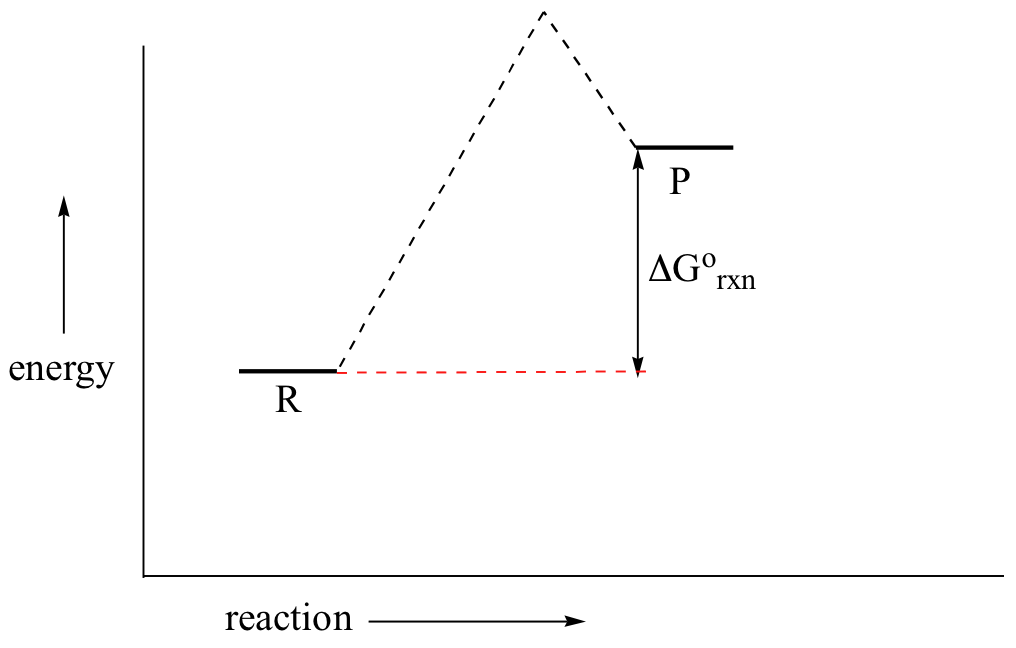
In a hypothetical endergonic (energy-absorbing) reaction the products would have a higher energy than reactants and thus ΔG˚rnx would be positive and Keq would be less than 1, favoring reactants.

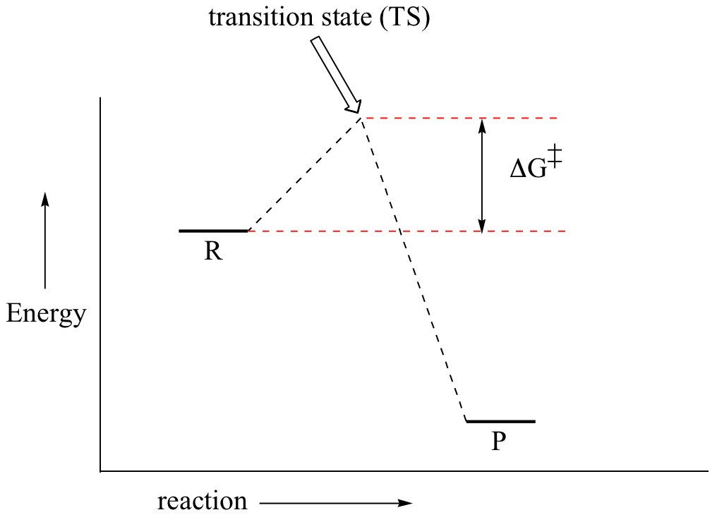
Now, let's move to kinetics. Look again at the energy diagram for exergonic reaction: although it is ‘downhill’ overall, it isn’t a straight downhill run.

First, an ‘energy barrier’ must be overcome to get to the product side. The height of this energy barrier, you may recall, is called the ‘activation energy’ (ΔG‡). The activation energy is what determines the kinetics of a reaction: the higher the energy hill, the slower the reaction. At the very top of the energy barrier, the reaction is at its transition state (TS), which is the point at which the bonds are in the process of breaking and forming. The transition state is an ‘activated complex’: a transient and dynamic state that, unlike more stable species, does not have any definable lifetime. It may help to imagine a transition state as being analogous to the exact moment that a baseball is struck by a bat. Transition states are drawn with dotted lines representing bonds that are in the process of breaking or forming, and the drawing is often enclosed by brackets. Here is a picture of a likely transition state for a substitution reaction between hydroxide and chloromethane:
\[CH_3Cl + HO^- \rightarrow CH_3OH + Cl^-\]

This reaction involves a collision between two molecules: for this reason, we say that it has second order kinetics. The rate expression for this type of reaction is:
rate = k[reactant 1][reactant 2]
. . . which tells us that the rate of the reaction depends on the rate constant k as well as on the concentration of both reactants. The rate constant can be determined experimentally by measuring the rate of the reaction with different starting reactant concentrations. The rate constant depends on the activation energy, of course, but also on temperature: a higher temperature means a higher k and a faster reaction, all else being equal. This should make intuitive sense: when there is more heat energy in the system, more of the reactant molecules are able to get over the energy barrier.
Here is one more interesting and useful expression. Consider a simple reaction where the reactants are A and B, and the product is AB (this is referred to as a condensation reaction, because two molecules are coming together, or condensing). If we know the rate constant k for the forward reaction and the rate constant kreverse for the reverse reaction (where AB splits apart into A and B), we can simply take the quotient to find our equilibrium constant \(K_{eq}\):
![]()
This too should make some intuitive sense; if the forward rate constant is higher than the reverse rate constant, equilibrium should lie towards products.

