27.3: Use of the Uncertainty Principle to Measure the Rates of Chemical Transformations
- Page ID
- 22378
\( \newcommand{\vecs}[1]{\overset { \scriptstyle \rightharpoonup} {\mathbf{#1}} } \)
\( \newcommand{\vecd}[1]{\overset{-\!-\!\rightharpoonup}{\vphantom{a}\smash {#1}}} \)
\( \newcommand{\id}{\mathrm{id}}\) \( \newcommand{\Span}{\mathrm{span}}\)
( \newcommand{\kernel}{\mathrm{null}\,}\) \( \newcommand{\range}{\mathrm{range}\,}\)
\( \newcommand{\RealPart}{\mathrm{Re}}\) \( \newcommand{\ImaginaryPart}{\mathrm{Im}}\)
\( \newcommand{\Argument}{\mathrm{Arg}}\) \( \newcommand{\norm}[1]{\| #1 \|}\)
\( \newcommand{\inner}[2]{\langle #1, #2 \rangle}\)
\( \newcommand{\Span}{\mathrm{span}}\)
\( \newcommand{\id}{\mathrm{id}}\)
\( \newcommand{\Span}{\mathrm{span}}\)
\( \newcommand{\kernel}{\mathrm{null}\,}\)
\( \newcommand{\range}{\mathrm{range}\,}\)
\( \newcommand{\RealPart}{\mathrm{Re}}\)
\( \newcommand{\ImaginaryPart}{\mathrm{Im}}\)
\( \newcommand{\Argument}{\mathrm{Arg}}\)
\( \newcommand{\norm}[1]{\| #1 \|}\)
\( \newcommand{\inner}[2]{\langle #1, #2 \rangle}\)
\( \newcommand{\Span}{\mathrm{span}}\) \( \newcommand{\AA}{\unicode[.8,0]{x212B}}\)
\( \newcommand{\vectorA}[1]{\vec{#1}} % arrow\)
\( \newcommand{\vectorAt}[1]{\vec{\text{#1}}} % arrow\)
\( \newcommand{\vectorB}[1]{\overset { \scriptstyle \rightharpoonup} {\mathbf{#1}} } \)
\( \newcommand{\vectorC}[1]{\textbf{#1}} \)
\( \newcommand{\vectorD}[1]{\overrightarrow{#1}} \)
\( \newcommand{\vectorDt}[1]{\overrightarrow{\text{#1}}} \)
\( \newcommand{\vectE}[1]{\overset{-\!-\!\rightharpoonup}{\vphantom{a}\smash{\mathbf {#1}}}} \)
\( \newcommand{\vecs}[1]{\overset { \scriptstyle \rightharpoonup} {\mathbf{#1}} } \)
\( \newcommand{\vecd}[1]{\overset{-\!-\!\rightharpoonup}{\vphantom{a}\smash {#1}}} \)
\(\newcommand{\avec}{\mathbf a}\) \(\newcommand{\bvec}{\mathbf b}\) \(\newcommand{\cvec}{\mathbf c}\) \(\newcommand{\dvec}{\mathbf d}\) \(\newcommand{\dtil}{\widetilde{\mathbf d}}\) \(\newcommand{\evec}{\mathbf e}\) \(\newcommand{\fvec}{\mathbf f}\) \(\newcommand{\nvec}{\mathbf n}\) \(\newcommand{\pvec}{\mathbf p}\) \(\newcommand{\qvec}{\mathbf q}\) \(\newcommand{\svec}{\mathbf s}\) \(\newcommand{\tvec}{\mathbf t}\) \(\newcommand{\uvec}{\mathbf u}\) \(\newcommand{\vvec}{\mathbf v}\) \(\newcommand{\wvec}{\mathbf w}\) \(\newcommand{\xvec}{\mathbf x}\) \(\newcommand{\yvec}{\mathbf y}\) \(\newcommand{\zvec}{\mathbf z}\) \(\newcommand{\rvec}{\mathbf r}\) \(\newcommand{\mvec}{\mathbf m}\) \(\newcommand{\zerovec}{\mathbf 0}\) \(\newcommand{\onevec}{\mathbf 1}\) \(\newcommand{\real}{\mathbb R}\) \(\newcommand{\twovec}[2]{\left[\begin{array}{r}#1 \\ #2 \end{array}\right]}\) \(\newcommand{\ctwovec}[2]{\left[\begin{array}{c}#1 \\ #2 \end{array}\right]}\) \(\newcommand{\threevec}[3]{\left[\begin{array}{r}#1 \\ #2 \\ #3 \end{array}\right]}\) \(\newcommand{\cthreevec}[3]{\left[\begin{array}{c}#1 \\ #2 \\ #3 \end{array}\right]}\) \(\newcommand{\fourvec}[4]{\left[\begin{array}{r}#1 \\ #2 \\ #3 \\ #4 \end{array}\right]}\) \(\newcommand{\cfourvec}[4]{\left[\begin{array}{c}#1 \\ #2 \\ #3 \\ #4 \end{array}\right]}\) \(\newcommand{\fivevec}[5]{\left[\begin{array}{r}#1 \\ #2 \\ #3 \\ #4 \\ #5 \\ \end{array}\right]}\) \(\newcommand{\cfivevec}[5]{\left[\begin{array}{c}#1 \\ #2 \\ #3 \\ #4 \\ #5 \\ \end{array}\right]}\) \(\newcommand{\mattwo}[4]{\left[\begin{array}{rr}#1 \amp #2 \\ #3 \amp #4 \\ \end{array}\right]}\) \(\newcommand{\laspan}[1]{\text{Span}\{#1\}}\) \(\newcommand{\bcal}{\cal B}\) \(\newcommand{\ccal}{\cal C}\) \(\newcommand{\scal}{\cal S}\) \(\newcommand{\wcal}{\cal W}\) \(\newcommand{\ecal}{\cal E}\) \(\newcommand{\coords}[2]{\left\{#1\right\}_{#2}}\) \(\newcommand{\gray}[1]{\color{gray}{#1}}\) \(\newcommand{\lgray}[1]{\color{lightgray}{#1}}\) \(\newcommand{\rank}{\operatorname{rank}}\) \(\newcommand{\row}{\text{Row}}\) \(\newcommand{\col}{\text{Col}}\) \(\renewcommand{\row}{\text{Row}}\) \(\newcommand{\nul}{\text{Nul}}\) \(\newcommand{\var}{\text{Var}}\) \(\newcommand{\corr}{\text{corr}}\) \(\newcommand{\len}[1]{\left|#1\right|}\) \(\newcommand{\bbar}{\overline{\bvec}}\) \(\newcommand{\bhat}{\widehat{\bvec}}\) \(\newcommand{\bperp}{\bvec^\perp}\) \(\newcommand{\xhat}{\widehat{\xvec}}\) \(\newcommand{\vhat}{\widehat{\vvec}}\) \(\newcommand{\uhat}{\widehat{\uvec}}\) \(\newcommand{\what}{\widehat{\wvec}}\) \(\newcommand{\Sighat}{\widehat{\Sigma}}\) \(\newcommand{\lt}{<}\) \(\newcommand{\gt}{>}\) \(\newcommand{\amp}{&}\) \(\definecolor{fillinmathshade}{gray}{0.9}\)We have seen how the uncertainty principle relates the attainable line widths in different kinds of spectroscopy to the lifetimes of the states - the shorter the lifetime, the greater the spread in energy of the states and the greater the spectroscopic line width. So far we have associated short lifetimes with excited states, but this need not necessarily be so. Short lifetimes also may be associated with chemical or conformational changes. As a specific example, suppose we have a magnetic nucleus in the \(+\frac{1}{2}\) state located in a chemical environment whereby it experiences a magnetic field \(H\) such that \(H = H_0 \left( 1 - \sigma \right)\). This nucleus will have a particular magnetic energy, call it \(E\). Now suppose the nucleus has a lifetime \(\Delta t\) before it moves to a different chemical environment where it experiences a different field \(H' = H_0 \left( 1 - \sigma' \right)\) and has a different energy \(E'\). Clearly, there will be an uncertainty in the energy \(E\) depending on the lifetime of the \(+\frac{1}{2}\) nucleus in the particular chemical environment before it switches to the new environment with a different shielding and a different energy.
Consider a specific example, 2,2,3,3-tetrachlorobutane. This substance can exist in three different conformations, \(1\), \(2\), and \(3\). By reference to the discussions in Section 5-2, you will recognize that \(1\) is achiral, whereas \(2\) and \(3\) are enantiomers:

Clearly, if we could separate \(1\) from \(2\) and \(3\), the protons of its methyl groups would have different chemical shifts from those of \(2\) and \(3\) (which, as enantiomers, would have their methyl proton resonances at the same frequency).
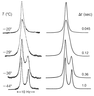
Now consider a mixture of the conformations \(1\), \(2\), and \(3\) in which the lifetimes of the conformations before they convert one into the other are \(\Delta t\). Assuming that the lifetimes of the \(+\frac{1}{2}\) and \(-\frac{1}{2}\) magnetic states are long compared to \(\Delta t\), then uncertainty in the transition energies will depend on the lifetimes of the chemical states (conformations) with different chemical shifts for the protons. The chemical-shift difference between \(1\) and \(2\) or \(3\) at \(-44^\text{o}\), as shown by Figure 27-3, is about \(5 \: \text{Hz}\). From Equation 27-1, we can see that \(5 \: \text{Hz}\) also will be the degree of the uncertainty in the frequency when \(\Delta t \sim 1/ \left( 2 \pi \Delta \nu \right) = 1/ \left( 2 \pi \times 5 \: \text{Hz} \right) = 0.03 \: \text{sec}\). Thus if \(1\) has a lifetime much longer than \(0.03 \: \text{sec}\), say \(1 \: \text{sec}\), before going to \(2\) or \(3\), it will give a sharp resonance of its own and, of course, \(2\) and \(3\) will also. However, if \(1\), \(2\), and \(3\) have lifetimes much shorter than \(0.03 \: \text{sec}\), say \(0.001 \: \text{sec}\), then we expect one average resonance for \(1\), \(2\), and \(3\).

Either condition can be realized for 2,2,3,3-tetrachlorobutane by taking the proton nmr spectrum at different temperatures (Figure 27-3). At \(-44^\text{o}\), at which \(\Delta t\) is \(1.0 \: \text{sec}\), we see the separate peaks for \(1\) and for \(2\) and \(3\). At \(-20^\text{o}\), at which \(\Delta t\) is \(0.045 \: \text{sec}\), the uncertainty is such that the lines have coalesced and we no longer can see the separate peaks. When the spectrum is taken at room temperature, at which \(\Delta t\) is about \(0.00005 \: \text{sec}\), a single very sharp line is observed. We get a sharp line at this temperature because, for practical purposes, there is no uncertainty about the average chemical shift of \(1\), \(2\), and \(3\). The line width now is determined again by the lifetimes of the \(+\frac{1}{2}\) and \(-\frac{1}{2}\) magnetic states, not by the lifetimes of the conformations.
Contributors and Attributions
John D. Robert and Marjorie C. Caserio (1977) Basic Principles of Organic Chemistry, second edition. W. A. Benjamin, Inc. , Menlo Park, CA. ISBN 0-8053-8329-8. This content is copyrighted under the following conditions, "You are granted permission for individual, educational, research and non-commercial reproduction, distribution, display and performance of this work in any format."


