1.6: Equations and graphs

Equalities where both sides have a single term, i.e., monomial, lead to the conversion factors. If one or both sides of the equality have more than one term, i.e., polynomial, it leads to a formula that does the same job, i.e., to convert units. Temperature conversion equations and ideal gas equations and the manipulation procedure of these equations are described below as examples of how to manipulate the questions needed for making calculations.

Temperature conversion equations

There are three temperature scales in common use: Celsius (^oC), Kelvin (K), and Fahrenheit (^oF), illustrated in Fig. 1.6.1.

Figure \(\PageIndex{1}\): Relations among temperature scales in common use. Source: MikeRun / CC BY-SA (https://creativecommons.org/licenses/by-sa/4.0)

Celsius (^oC)

The Celsius scale has O ^oC at the freezing point of water and 100 ^oC at the boiling point of water. Celsius is the base unit of temperature in the metric system.

The Kelvin scale

Kelvin is the base unit of temperature in the SI. The freezing point of water is 273.15 K, and the boiling point of water is 373.15 K. For most practical purposes, the freezing point of water is reported as 273 K and the boiling point 373 K, i.e., accurate to three significant figures. Celsius scale units are the same size but shifted up by 273 compared to the Kelvin scale. So, the relationship between Kelvin and Celsius is:

\begin{equation}
T_{K}= T_{C}+273,\nonumber
\end{equation}

where T_K is the temperature in Kelvin, and T_C is the temperature in degrees Celsius. This equation converts temperature in Kelvin to temperature in Celsius.

A 0 K, also called absolute zero, is the temperature of a matter at which no energy can be removed as heat from the matter. There is no negative temperature on the Kelvin scale.

Fahrenheit (^oF)

Fahrenheit is the base unit of the English system, with 32 ^oF at the freezing point of water and 212 ^oF at the boiling point of water. Fahrenheit is \(\frac{5}{9}\) times shorter and shifted up by 32 than Celsius. So the relationship between the two is:

\begin{equation}
T_{F}=\frac{9}{5} \times T_{C}+32,\nonumber
\end{equation}

where T_F is the temperature in Fahrenheit, and T_C is the temperature in degrees Celsius. This equation converts temperature in Celsius to temperature in Fahrenheit.

Manipulating temperature conversion equations

The equation for converting Celsius to Fahrenheit is:

\begin{equation}
T_{F}=\frac{9}{5} \times T_{C}+32,\nonumber
\end{equation}

Addition or subtraction of the same number on the two sides of an equation does not change the equality. Subtracting 32 from both sides of the above equation leads to:

\begin{equation}
T_{F} -32=\frac{9}{5} \times T_{C}\cancel{+32}\cancel{-32},\nonumber
\end{equation}

\begin{equation}
T_{F} -32=\frac{9}{5} \times T_{C}.\nonumber
\end{equation}

Multiplication or division by the same number on both sides of an equation does not change equality. Remember that multiplication or division should apply to every term on either side of the equality. Enclose the side with more than one term in small brackets and then do the multiplication of division operation so that it applies to each term in the bracket. Multiplying both sides of the above equation with \(\frac{5}{9}\) leads to:

\begin{equation}
\frac{5}{9} \times\left(T_{F}-32\right)=\cancel{\frac{5}{9}} \times \cancel{\frac{9}{5}} \times T_{C}\nonumber
\end{equation}

\begin{equation}
\frac{5}{9} \times\left(T_{F}-32\right)=T_{C}\nonumber
\end{equation}

Swapping the sides of an equation does not change equality. Swapping the sides in the above equation to bring T_C to the left:

\begin{equation}
T_{C}=\frac{5}{9} \times\left(T_{F}-32\right)\nonumber
\end{equation}

This is the equation for Fahrenheit to Celsius conversion.

The procedure of rearranging an equation described above applies to all algebraic equations. For example, start with a relationship that converts Celsius to Kelvin:

\begin{equation}
T_{K}= T_{C}+273,\nonumber
\end{equation}

subtract 273 from both sides:

\begin{equation}
T_{K}-273= T_{C}\cancel{+273}\cancel{-273},\nonumber
\end{equation}

\begin{equation}
T_{K}-273= T_{C},\nonumber
\end{equation}

and finally swap the left and right side to bring T_C to the left:

\begin{equation}
T_{C}=T_{K}-273.\nonumber
\end{equation}

This is the equation for Kelvin to Celsius conversion.

Ideal gas equation

The ideal gas equation relates more than two variables:

\[PV=nRT,\nonumber\]

where P is pressure, V is volume, n is the amount of gas in moles, T is the temperature (in K), and R is the proportionality constant called an ideal gas constant. Dividing both sides of the equation with V leads to:

\[P\times\frac{V}{V}=\frac{nRT}{V},\nonumber\]

\[P=\frac{n R T}{V}.\nonumber\]

It allows calculating the pressure of a gas sample if the amount in moles, temperature in kelvin, and volume of the gas sample are known, along with the value of the constant R in the consistent units. Similarly, rearranging the equation leads to formulas for calculating, V, T or n of a gas sample:

\begin{equation}
V=\frac{n R T}{P}, \quad T=\frac{P V}{n R}, \quad \text { and } \quad n=\frac{P V}{R T}\nonumber
\end{equation}

Graphs

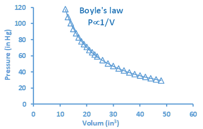
The graph is a visual presentation of a relationship between two variables. Fig. 1.6.2 shows a graph that presents a relationship between the volume and pressure of a given amount of gas at a constant temperature, known as Boyle’s law.

Figure \(\PageIndex{2}\): Boyle’s law –the relationship between pressure and volume of a given amount of gas at a constant temperature.

The typical components of a graph are the following.

1. A title that tells what the graph is about, e.g., “Boyle’s Law: ” in the graph of Fig. 1.6.2.
2. Axes: the x-axis is a horizontal line, and the y-axis is a vertical line. Axes usually have an evenly distributed scale starting from zero. The x-axis represents the independent variable, and the y-axis represents the dependent variable. For example, volume is independent, and pressure is the dependent variable in Fig. 1.6.2.
3. Axes labels that tell the variable's name and the units of measurement. For example, volume (in³) and pressure (in Hg), where in³ and in Hg are the units of the variables.
4. Symbols representing experimental points. For example, ∆ symbols in Fig 1.6.2, at the crossing of a vertical line starting from an experimental value independent variable on the x-axis and a horizontal line starting from the corresponding value of the dependent variable on the y-axis.
5. A curve connects the experimental points and shows the trend in the relationship. For example, the cure in Fig. 1.6.2 tells that the pressure decreases as the volume increases.

Interpretation of a graph

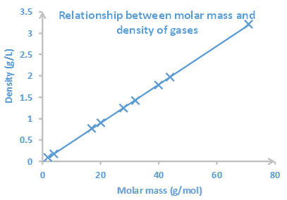
Interpretation is reading the trend or relationship between the variables plotted. For example, Fig. 1.6.2 shows that the pressure decreases as the volume of gas increases. The curve also allows reading the value of one variable from the value of the other. For example, if the volume is 30 in³, the pressure would be ~50 in Hg. To read: draw a vertical line from the given value on the x-axis and a horizontal line from the point where the vertical line crosses the curve. Then, read the value where the horizontal line meets the y-axis. The process is reversed when the given value is of the dependent variable on the y-axis, and the desired is the corresponding value of the independent variable on the x-axis. For example, if the pressure is 40 in Hg, the volume is about 35 in³. Fig. 1.6.3 is another example of a graph that shows a relationship between the molar mass and density of the gases at a constant temperature. The cure in this graph tells that the density of gases increases as the molar mass increases.

Figure \(\PageIndex{3}\): Curve showing gases having lower molar masses are less dense at the same temperature.