1.6: SALCs and the projection operator technique

SALCs refers to Symmetry Adapted Linear Combinations, which are generated via use of the projection operator technique. This technique is a mathematical method which outputs a function called a SALC that models the orbitals of the atoms of interest.^[1] These SALCs are mathematical representations and therefore bare no physical meaning. They are commonly used in the generation of molecular orbitals.

Projection Operator Technique

The Projection Operator Technique utilizes the extended character table which includes each symmetry operation separately. The technique involves multiple steps, listed below in the form of the \(\ce{BF_3}\) example.

Step 1. We begin by determining the reducible representations of the orbitals in question. For BF₃, which has the D_3h point group, the D_3h character table is used. For our example, we will consider the sigma and pi bonds of the fluorine atoms and determine their reducible representations. Using the character table, we identify the reducible representations. They are listed below.

\[\begin{align*} Γ_σ &= Α1^\prime + Ε^\prime \\[4pt] Γ_{πx} &= Α2^\prime + Ε^\prime \\[4pt] Γ_{πy} &= Α2^{\prime\prime} + Ε^{\prime\prime} \\[4pt] Γ_{πz} &= Α1^{\prime} + Ε^{\prime} \end{align*} \]

It is noted here that the \(π_z\) orbitals transform as \(σ\) orbitals.

Table \(\PageIndex{1}\). This is the character table for the \(D_{3h}\) point group which can be used to determine the irreducible representations of the orbitals.

D3h	E	C3	C2	σh	S3	σv
A1'	1	1	1	1	1	1
A2'	1	1	-1	1	1	-1
E'	2	-1	0	2	-1	0
A1"	1	1	1	-1	-1	-1
A2"	1	1	-1	-1	-1	1
E"	2	-1	0	-2	1	0

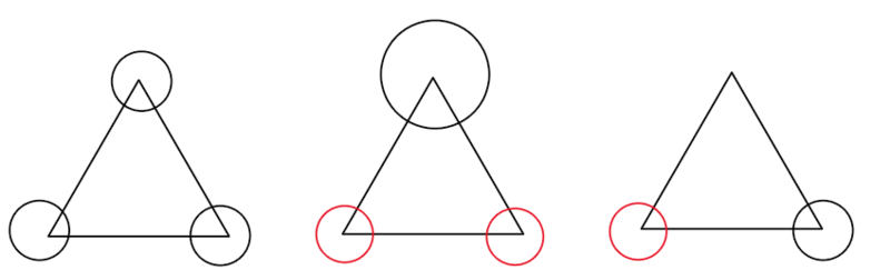
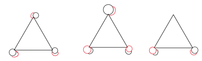
Step 2. We now use the extended character table for the D_3h Character table to generate the SALCs of the stated orbitals. To do this, we apply each symmetry operation to the given orbital and note which orbital it transforms into. We then add up each projector operator function in accordance to each irreducible representation.

Table \(\PageIndex{2}\). This is the extended character table for the D3h point group which is used to deduce the functions for the SALCs using the projector operator technique.

D3h	E	C3	C3^2	C2	C2^'	C2^"	σh	S3
Γσ	σ1	σ2	σ3	σ1	σ2	σ3	σ1	σ2
Γπz	\(\pi_{1}\)	\(\pi_{2}\)	\(\pi_{3}\)	\(\pi_{1}\)	\(\pi_{2}\)	\(\pi_{3}\)	\(\pi_{1}\)	\(\pi_{2}\)
Γπx	\(\pi_{1}\)	\(\pi_{2}\)	\(\pi_{3}\)	\(-\pi_{1}\)	\(-\pi_{2}\)	\(-\pi_{3}\)	\(\pi_{1}\)	\(\pi_{2}\)
Γπy	\(\pi_{1}\)	\(\pi_{2}\)	\(\pi_{3}\)	\(-\pi_{1}\)	\(-\pi_{2}\)	\(-\pi_{3}\)	\(-\pi_{1}\)	\(-\pi_{2}\)

Step 3. Common techniques for dealing with the double degeneracy of the E' and E" representations^[2]:

1. If the principal axis is a C₃ axis, we subtract the functions corresponding to the σ₂ and σ₃ orbitals.
2. If the principal axis is a C₄ axis, we apply the projection operator technique to the σ₂ and use the function that is derived.
3. We must ensure that the representations are orthogonal to one another in order for them to be correct.

Step 4. We can now apply the coefficients within the matrix to determine the coefficients of the function found via the projection operator technique.

We determine the SALCs for the example orbitals to be the following:

\[\begin{align*} \text{SALC}_σ(A_1') &= 3σ_1 + 3σ_2 + 3σ_3 = σ_1 + σ_2 + σ_3 \\[4pt] \text{SALC}_σ(E') &= 4σ_1 - 2σ_2 - 2σ_3 = 2σ_1 - σ_2 - σ_3 \\[4pt] \text{SALC}_σ(E') &= 2σ_2 - 2σ_3 = σ_2 - σ_3 \end{align*} \]

Figure \(\PageIndex{1}\). This is a rendering of the SALCs for the sigma orbitals of the fluorine atoms of BF3. From left to right, the A1', E', and E' SALCs are depicted.

\[\begin{align*} \text{SALC}_{πz}(A_1') &= 3π_1 + 3π_2 + 3π_3 = π_1 + π_2 + π_3 \\[4pt] \text{SALC}_{πz}(E') &= 4π_1 - 2π_2 - 2π_3 = 2π_1 - π_2 - π_3 \\[4pt] \text{SALC}_{πz}(E') &= 2π_2 - 2π_3 = π_2 - π_3 \end{align*} \]

Figure \(\PageIndex{2}\): This is a rendering of the SALCs for the pi-z orbitals of the fluorine atoms of BF₃. From left to right, the A1', E', and E' SALCs are depicted.

\[\begin{align*} \text{SALC}_{πx}(A_2') &= 3π_1 + 3π_2 + 3π_3 = π_1 + π_2 + π_3 \\[4pt] \text{SALC}_{πx}(E') &= 4π_1 - 2π_2 - 2π_3 = 2π_1 - π_2 - π-3 \\[4pt] \text{SALC}_{πx}(E') &= 2π_2 - 2π_3 = π_2 - π_3 \end{align*} \]

Figure \(\PageIndex{3}\): This is a rendering of the SALCs for the pi-x orbitals of the fluorine atoms of BF₃. From left to right, the A2', E', and E' SALCs are depicted.

\[\begin{align*} \text{SALC}_{πy}(A_2'') &= 3π_1 + 3π_2 + 3π_3 = π_1 + π_2 + π_3 \\[4pt] \text{SALC}_{πy}(E'') &= 4π_1 - 2π_2 - 2π_3 = 2π_1 - π_2 - π_3 \\[4pt] \text{SALC}_{πy}(E'') &= 2π_2 - 2π_3 = π_2 - π_3 \end{align*} \]

Figure \(\PageIndex{4}\). This is a rendering of the SALCs for the pi-y orbitals of the fluorine atoms of BF3. From left to right, the A2", E", and E" SALCs are depicted.

Uses of SALCs

SALCs help us to understand which orbitals will be bonding, antibonding, and nonbonding. For example, by comparing the symmetry of the SALCs to that of the orbitals of the central atom, it is possible to generate the corresponding molecular orbitals. Although SALCs are mathematical representations that have no physical meaning, they are useful in providing a tool for deriving molecular orbitals.

References

1. www4.ncsu.edu/~franzen/public...ojection_1.pdf
2. http://troglerlab.ucsd.edu/GroupTheory224/Chap2B.pdf