3.2: The Symmetry Adapted Linear Combination of Atomic Orbitals Method

Rules for the Symmetry-Adapted Linear Combination of Atomic Orbitals (SALC)

The construction of molecular orbitals using group theory follows a method called “Symmetry-adapted linear combination of atomic orbitals”. This method follows the following steps.

1. Firstly, we determine the point group for the molecule.
2. Secondly, we determine the axes of the coordinate system in a useful way.
3. Thirdly, we determine the ligand atomic orbitals that can be combined to form so-called ligand group orbitals (LGOs). These are usually orbitals of the same kind that a symmetry operation can interconvert. The number of LGOs is always the number of the ligand atomic orbitals.
4. In the next step, we determine the symmetry types of the ligand group orbitals, and we will talk in a moment how this works.
5. Finally, we determine the symmetry type of the atomic orbitals of our central atom, and combine ligand group orbitals and central atom orbitals of the same symmetry type. If they have the same symmetry type their symmetry is “right”. The MOs resulting from this combination will have the same symmetry type as the orbitals from which they have been made. Also the number of MOs must be the same as the number of LGOs and central atom AOs.

Now you can construct a molecular orbitals diagram using the MOs that you have constructed using SALC. After you have constructed the MO diagram, always check that the number of MOs is equal to the number of AOs. If not, you must have made a mistake and you have to go back and find the mistake.

Example - H₂O

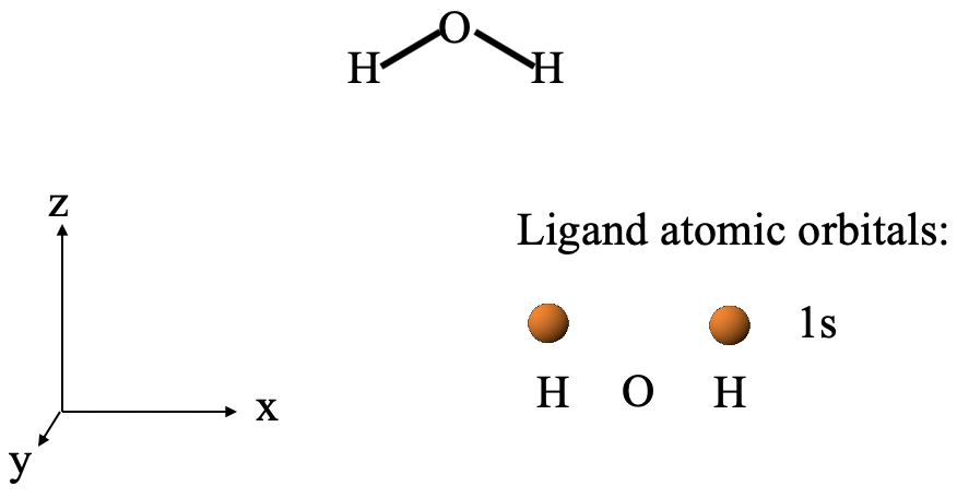
Let us carry out these steps using our water molecule as an example. As we determined previously, the point group of the water molecule is C_2v. A sensible way to define the coordinate system is to have the x-axis point to the right, the z-axis point to the top, and the y-axis point out of the paper plane (Fig. 3.2.1). The water molecule would be in the xz plane pointing into z-direction. The next step is to define the ligand atoms and ligand orbitals. It is easy to see that the H atoms would be ligand atoms, and the O atom would be the central atom. The ligand atomic orbitals that would be combined to form ligand group orbitals would be the 1s orbitals of the hydrogen atoms. We would expect two ligand group orbitals because we combine two atomic orbitals.

Figure 3.2.1 SALC for the water molecule (step 1 and 2)

Determination of LGO Symmetry Types

Next, we need to determine the symmetry types of the ligand group orbitals (LGOs). We can do this in two steps.

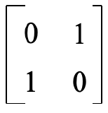
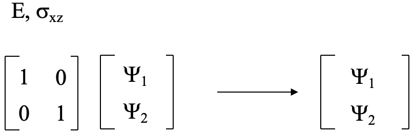
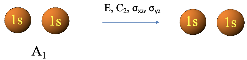
In the first step, we determine the reducible representation for the ligand group orbitals by a method called the “orbital swapping method”, and in the second step we determine the irreducible representations for the ligand group orbitals from the reducible representation. The irreducible representations will give us the symmetry type of the ligand group orbitals. Let us do the first step, and carry out the orbitals swapping method to determine the reducible representation. To do so, let us first denote the two 1s orbitals Ψ1 and Ψ2, respectively (Fig. 3.2.2).

Figure 3.2.2 The 1s orbitals of the hydrogen atoms of the water molecule denoted as Ψ1 and Ψ2

Then, we decide if Ψ1 and Ψ2 get swapped up when a particular symmetry operation is carried out. If so, each gets a character zero, if not, they get a character +1 each. The sum of these characters give the character in the reducible representation for the particular symmetry operation. After we have applied orbital swapping for all symmetry operations, we know all the characters of the reducible representation. The E symmetry operation does not swap the orbitals, hence the character in the reducible representation is 1+1=2 (Fig. 3.2.3). The C₂ symmetry operation does swap the orbitals, hence the character in the reducible representation is 0+0=0. The xz mirror plane leaves the orbitals at their positions, therefore the character in the reducible representation is 1+1=2. the yz mirror plane swaps the orbitals, hence the character is 0+0=0 (Fig. 2.3.2).

Figure 3.2.3 Using the orbital swapping method to determine the reducible representation for the LGOs of the water molecule

You may ask: Why does the orbital swapping method work? What deeper principle is behind it? The answer is. The orbital swapping method is a short-cut for getting the sum of the characters on the trace of a transformation matrix that converts the two wave functions. Before the symmetry operation is carried out the two wave functions can be described by a matrix of of the form below (Fig. 3.2.4).

Figure 3.2.4 Matrix that represents the two 1s orbitals.

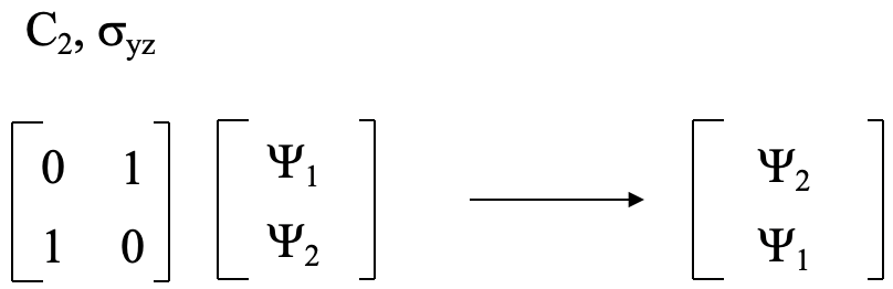
When the orbitals are swapped, Ψ1 and Ψ2 on the matrix are swapped, and the matrix takes the form below (Fig. 3.2.5).

Figure 3.2.5 Matrix that represents the two 1s orbitals after the orbitals haven been swapped

The transformation matrix when multiplied with the matrix in Figure 3.2.4 gives the matrix in Figure 3.2.5 which is the transformation matrix for the operation(s). This matrix has the form below (Fig. 3.2.6),

Figure 3.2.6 The transformation matrix for C₂ and σ_yz

and we could use the multiplication rules to show that this matrix is the correct matrix. This means the transformation matrix for C₂ and σ_yz is the matrix shown in Figure 3.2.6.

Figure 3.2.7 Multiplication of the matrix representing the 1s orbitals with the matrix representation for C₂ and σ_yz

For the operations E and σ_xz the orbitals do not get swapped, and the final matrix is the same as the initial matrix in Figure 3.2.4. Thus, the transformation matrix has the form below (Fig. 3.2.8). For the matrix in Figure 3.2.6 the sum of the characters on the trace of the matrix is zero. For the matrix below

Figure 3.2.8 Transformation matrix for E and σ_xz

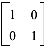
this sum is 2. These are the characters of the reducible representation that we previously determined using the orbital swapping method. Using the multiplication rules we can show that the matrix of Fig. 3.2.8 is the correct transformation matrix (Fig. 3.2.9)

Figure 3.2.9 Multiplication of the matrix for the 1s orbitals with the matrix representation for E and σ_xz

In the next step we need to determine the irreducible representations from the reducible representation. Remember, a reducible representation is the sum of two or more irreducible representations. Thus, a reducible representation contains the information about the irreducible representations it is composed of, and we need to find a tool to extract that information.

The tool to do this is a formula from group theory called the reduction formula. You can see the reduction formula below (Fig. 3.2.10).

Figure 3.2.10 The reduction formula

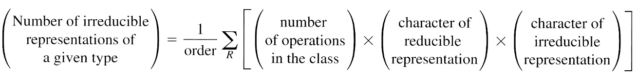
It says that the number of irreducible representations of a given symmetry type is one over the order of the point group times the sum of the products of the number of operations in a specific class in the character table of the point group times the character of the reducible representation for a given symmetry operation times the character of the irreducible representation for a given symmetry operation. The "sum of products" means the sum of the products for all classes of symmetry operations in the point group. The number of operations in a class and the character of the irreducible representation can be read from the character table for the point group. Here we see for the first time the utility of character tables for molecular orbital theory. The characters of the reducible representation can be read from the reducible representation previously determined by the orbital swapping method.

Figure 3.2.11 The reducible representation of the LGOs of the water molecule and the character table of C_2v

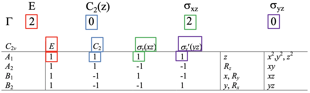
For clarity, let us use the reduction formula for the determination of the irreducible representations of the ligand group orbitals for the example of the water molecule. Our task is to find the number of irreducible representations of each possible symmetry type in the point group. In the point group C_2v, these are the symmetry types A₁, A₂, B₁, and B₂. Let us start with A₁. The number of irreducible representations of the type A₁ is: A₁ = 1/4 (1x2x1 + 1x0x1 + 1x2x1 + 1x0x1) = 1 (Fig. 3.2.12).

Figure 3.2.12 Calculation of the number of irreducible representations A₁

The result means that one of the two ligand group orbitals has the symmetry type A₁. The factor ¼ is because the order of the point group is 4. We can determine the order just by counting the number of symmetry operations in the character table for C_2v. The first product 1x2x1 (red) is the product for the identity E. The number of operations in the column for E is 1, there is never another conjugate operation in the class for the identity. Note that the number “1” is not explicitly spelled out. The number of operation within a class of a character table is only spelled out when the number is larger than 1. The character in the reducible representation for E is 2, and the character for the irreducible representation for the A₁ symmetry type underneath E is also 1. The second product is 1x0x1 (blue) because the number of operations in the class of for C₂ is 1, the character in the reducible representation for C₂ is 0, and the character of the irreducible representation underneath C₂ is 1. The third product for the σ_xz operation is 1x2x1 (green) because the character for the class σ_xz is 1, the character in the reducible representation for σ_xz is 2, and the character of the irreducible representation under σ_xz is 1. Lastly, the product for the operation σ_yz is 1x0x1 (black) because the number of operations in the class for σ_yz is 1, the character in the reducible representation under σ_yz is 0, and the character of the irreducible representation under σ_yz is 1 (purple).

Using the same procedure, we can also determine the number of ligand group orbitals that have the symmetry types, A₂, B₁, and B₂.

Figure 3.2.13 Calculation for the number of irreducible representations for A₂, B₁, and B₂, respectively

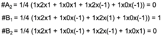
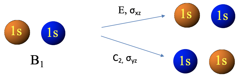
The result (Fig. 3.2.13) is that the second ligand group orbital has the symmetry type B₁, and the number of ligand group orbitals with the symmetry type A₂ and B₂ is 0. We have determined that the reducible representation is the sum of the two irreducible representations A₁ and B₂ (Fig. 3.2.14).

Figure 3.2.14 The reducible representation shown as the sum of the two irreducible representations

The result means that one ligand group orbital has A₁ symmetry, the other B₁ symmetry. The one with A₁ symmetry reflects the combination of two 1s orbitals with the same algebraic sign, the one with B₁ symmetry reflects the combination of two 1s orbitals with opposite algebraic sign.

We encountered the LGOs already previously by inspection. Here we see that group theory can formally derive them. We can also verify that the two LGOs have A₁ and B₁ symmetry, respectively, by carrying out the symmetry operations and see what they do to the respective LGO. For the LGO with A₁ symmetry, no symmetry operation changes the LGO (Fig. 3.2.15). This is consistent with the symmetry type A₁ for which all characters on the irreducible representation are 1.

Figure 3.2.15 Verifying the A₁ symmetry by carrying out the symmetry operations

For the LGO with B₁ symmetry type we see that the C₂ operation and the σ_yz operations reverse the algebraic sign of the wave function, while the identity and the σ_yz operations don’t (Fig. 3.2.16). This is consistent with the irreducible representation of the B₁ symmetry type which has the characters +1 for E and σ_xz, and -1 for the operations C₂ and σ_yz.

Figure 3.2.16 Verifying the B₁ symmetry of the second LGO by carrying out the symmetry operations

Symmetry Type Determination of Central Atom Orbitals

In the next step we have to find out the symmetry types of the central atom valence orbitals. In the case of the water molecule the central atom valence orbitals are the 2s, and the three 2p orbitals. We can easily read the symmetry types of these orbitals from the character table of the point group C_2v (Fig. 3.2.17).

Figure 3.2.17 The character table of the point group C_2v and the symmetry types of the central atom valence orbitals

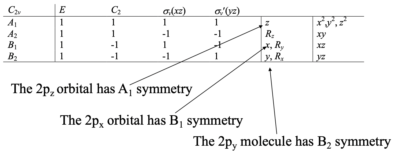
An s orbital is always of the totally symmetric symmetry type in the point group. This is the symmetry type with all characters having a +1 value. In the point group C_2v this is the symmetry type A₁. The symmetry type of the 2p_z orbital is also A₁. This is because the letter z is in the row for the symmetry type A₁. Similarly, the 2p_x and the 2p_y orbitals have the symmetry type B₁ and B₂ respectively because the letters x and y are in the rows for the symmetry types B₁ and B₂, respectively.

Combination of AOs and LGO to form MOs

When central atom AOs have the same symmetry type then they have the “right” symmetry to be combined to form molecular orbitals. The molecular orbitals will have the same symmetry type than the AOs and LGOs from which they have been made. The number of MOs of a specific symmetry type must be equal to the sum of the LGOs and AOs that have the same symmetry type. When an orbital does not find a partner orbital of the same symmetry type then it is non-bonding.

Let us apply these ideas to the example of the water molecule. We saw that there were two AOs that had the symmetry type A₁, namely the 2s and the 2p_z orbital. There was also an LGO with A₁ symmetry. We can therefore combine these three orbitals to form molecular orbitals. They also must have the symmetry type A₁ (Fig. 3.2.18).

Figure 3.2.18 Combination of A₁ AOs and LGOs to create MOs

Next, let us think about orbitals of the symmetry type A₂. No AO and no LGO has this symmetry type. Therefore, there are also no MOs of this symmetry type (Fig. 3.2.19).

Figure 3.2.19 AOs and LGOs of the A₂ symmetry type

For the symmetry type B₁ we find that there is one AO, namely the 2p_x orbital and one LGO that have this symmetry type. This means that these two orbitals can be combined to form two MOs of the same symmetry type (Fig. 3.2.20).

Figure 3.2.20 Combination of the AOs and LGOs of the B₁ symmetry type

For the B₂ symmetry there is only the 2p_y AO, but no LGO it could be combined with. Thus, the 2p_y orbital remains non-bonding (Fig. 3.2.21).

Figure 3.2.21 AOs and LGOs of the B₂ symmetry type

Remember, we got the same result when we analyzed the orbitals by inspection. Here, group theory give us the same result through a formalism. This has the advantage that ambiguity and mistakes are avoided. Nonetheless, it should be kept in mind what the group-theoretical result means, and for that it is useful to have previously analyzed the interactions of the 2p orbitals with the 1s orbitals by inspection.

The MO Diagram of H₂O

Now we can construct the molecular orbital diagram of H₂O. As always we first draw a vertical arrow for the energy axis (Fig 3.2.22). Next we indicate the atom symbols on the left and the right side of the diagram. By convention, the the central atom is on the left side. After that we can write the atomic orbitals into the molecular orbital diagram according to approximate relative energy, and indicate their names and symmetry.

Figure 3.2.22 MO diagram of H₂O and its relationship to the valence bond structure of H₂O

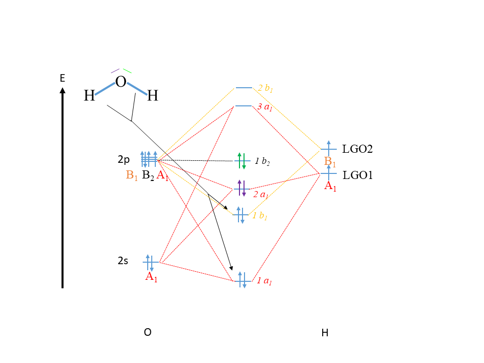
We know that the 2s orbitals of O must be lower in energy than the 2p orbitals of O, and we write them accordingly. We also know that the 2p orbitals all have the same energy, and so we write them together as close as possible. For the H orbitals we write the ligand group orbitals and indicate them LGO1 and LGO2. We do not know the exact energy of the LGOs relative to the 2p and 2s orbitals of oxygen, but we would expect that it is similar to the them, otherwise we could not make covalent bond. We also know that the O-H bonds are polarized toward O, so we would suspect that the LGOs are more similar to the 2p orbitals in energy compared to the 2s orbitals. We write the LGO2 somewhat above LGO1 to indicate the LGO2 has a slightly higher energy because it has a node. It is also ok though to write them out with the same energy, both methods are common in the literature. We indicate that LGO1 has the symmetry type A₁ and LGO2 has the symmetry type B₁.

Now we need to write out the molecular orbitals in the middle of the diagram. We go systematically through all the symmetry types as we construct the MOs. For example, we can start with the symmetry type A₁. Because we combine three orbitals of this symmetry type we need to write three MOs into the middle of the diagram, and indicate the symmetry type. When we combine three orbitals the following approximation holds. There will be one bonding orbital of low energy, one anti-bonding orbital of high energy, and a third one of intermediate energy that is approximately non-bonding. We do not know if it is exactly non-bonding, slightly bonding or slightly anti-bonding. Exact quantum-mechanical calculations could determine this as well as the exact energy of the orbital, but here our focus is on the qualitative construction and understanding of molecular orbital diagrams. Therefore, we must leave this question unanswered. The bonding orbital should be written below the lowest energy atomic orbital which contributes to the MO, in this case the 2s orbital of O. The anti-bonding orbital should be drawn at an energy level above the highest-energy orbital that contributes to it, in this case the A₁-type 2p orbital. You can draw the approximately non-bonding a₁-type MO at approximately half the distance between the bonding and the anti-bonding MO into the diagram. The lowest energy orbital gets the label 1a₁, the second-lowest, the label 2a₁, and the highest energy orbital gets the label 3a₁. Note that for the MOs we use lower case letters to indicate the symmetry type. The coefficients in front of the symmetry type numbers the orbitals according to increasing energy. In the last step we connect all A₁-type AOs and LGOs with the a₁-type MOs by dotted lines. This is indicated by the dotted, red lines in Fig. 3.2.22.

Next, we can draw the b₁-type MOs. We expect two MOs, because there is one AO of this symmetry type, and one LGO of this symmetry type. One MO is expected to be bonding and should have low energy, the other one must be anti-bonding, and have high energy. The energy of the bonding MO should be lower than the energy of the lowest energy orbital that contributes to it, in this case the B₁-type 2p orbital. The anti-bonding orbital should have a higher energy than the highest energy AO/LGO that contributes to it, in this case the LGO2. The bonding MO gets the label 1b₁ and the anti-bonding orbital the label 2b₁. We do not exactly know the energy of the b₁-type MOs relative to the a₁ type AOs when qualitatively drawing the MO diagram. For example, the anti-bonding 2b₁ orbital is drawn with a higher energy than the anti-bonding 3a₁ orbital, but we would not that for sure (only exact quantum-mechanical calculations could tell). We would however suspect, that the bonding 1b₁ orbital has a higher energy than the bonding 1a₁ orbital because the energy of the 2s orbital is significantly lower than the energy of the B₁-type 2p orbital. We would also suspect that the 1b₁ orbital is lower in energy than the 2a₁ orbital because we know that the 1b₁ is bonding, while the 2a₁ is approximately non-bonding. Finally, we connect the AOs and LGOs with B₁ symmetry with the MOs of b₁ symmetry with dotted lines, indicated orange in Fig. 3.2.22.

Lastly, we still have to decide what to do with the 2p_y orbital that has the symmetry type B₂. This orbital has no partner of the same symmetry type, and thus remains exactly non-bonding. Therefore, we write the 2p_y orbital as a b₂-type orbital with unchanged energy in the middle of the MO diagram, and interconnect the two orbitals with a horizontal, dotted line, Fig. 3.2.22.

Now let us fill the electrons into the orbitals. The O atom has six valence electrons, two of them are in the 2s orbitals and four of them are in the 2p orbitals. The 2p orbitals are filled according to Hund’s rule. Because each H atom contributes one electron, the LGOs are both considered half-full with one electron each. Now we can fill the MOs according to increasing energy. Overall we have 6+2=8 electrons to fill into the MOs. Consequently, the 1a₁ gets filled first, then the 1b₁, then the 2a₁, and finally the 1b₂. The 1b₂ is called the highest occupied molecular orbital, abbreviated HOMO. The next higher orbital, the 3a₁ orbital is called the lowest unoccupied orbital, also called LUMO. HOMOs and LUMO are important for the chemistry of a molecule because the HOMO electrons are the most reactive electrons, and the LUMO is the orbital that easiest to fill with an electron coming from a co-reactant.

Now our MO diagram is complete. It is insightful to compare the MO diagram of water with the Lewis-dot structure of the water molecule to understand what additional information we can gain from the MO diagram compared to the Lewis dot structure. In the Lewis dot structure there, are two localized O-H bonds, so overall we have four bonding electrons. Can we we see these bonding electrons also in the MO diagram? Well, we recognize that there are two bonding molecular orbitals that are filled, the 1a₁ and the 1b₁. Therefore, also in the MO diagram there are four bonding electrons. You can see however, that the two MOs are not energetically equal, thus two electrons have a higher energy than the other two. This is something that we do NOT see in the Lewis-dot structure. According to the Lewis dot structure all four electrons are equivalent. The bonding MOs in water are delocalized over the entire molecule. In contrast to that in the Lewis dot structure two electrons are localized in the first O-H bond, and the other two in the second O-H bond. This is another difference between the Lewis-dot and the MO picture of the covalent bonding in water.

Next, let us see if there is an equivalent of the two electron lone pairs at O in the Lewis dot structure in the MO diagram. We can see that there are two filled, non-bonding MOs, the 1b₂ is completely non-bonding, and the 2a₁ is approximately non-bonding. We can argue that these non-bonding electrons are the counterparts of the four electrons in the two electron lone pairs. However, in the Lewis-dot structure the two electron lone pairs appear equivalent. In the MO picture we can see that the two non-bonding electrons have a higher energy than the other two.

Overall, we can say that the MO diagrams gives us a more refined picture of the covalent bonding compared to the Lewis dot structure. This however comes at the price of constructing a complicated MO diagram compared to a simple Lewis dot structure. Therefore, our decision to construct or not construct an MO diagram depends on how much detail we need to know in the context of a chemical problem that we want to solve. For example, light absorption due to electron transitions cannot be explained via a Lewis-dot structure, we need an MO diagram to understand that.

The MO Diagram of NH₃

Let us do another, more complex example to enhance our understanding of MO theory, the example of the MO diagram of NH₃. The NH₃ molecule belongs to the point group C_3v. The coordinate system can be chosen so that the z-axis points vertically, and the x-axis points to the right. The y-axis stands perpendicular to the paper plane. The NH₃ molecule is oriented with the tip of the pyramid pointing up and one N-H bond being in the xz plane (Fig. 3.2.23).

Figure 3.2.23 The chosen coordinate system and the ligand orbitals of NH₃

We would choose the N atom as the central atom and the H atoms the ligand atoms. The relevant ligand orbitals for bonding would be the 1s orbital of the H atoms. We would group them to form ligand group orbitals. Three LGOs would be expected as three 1s orbitals would be combined.

The Reducible Representation of the LGOs of NH₃

The next step is to determine the reducible representation of the LGOs using the orbital swapping method, Fig. 3.2.24.

Figure 3.2.24 Orbital swapping method for the 1s LGOs of NH₃

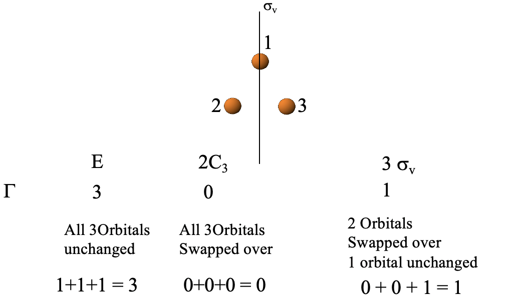
We can see that the identity leaves all three orbitals unchanged, hence the character on the reducible representation for E is 1+1+1=3 (Fig. 3.2.24).

Next we need to see what a C₃ operation does. It changes the position of all three orbitals, so the character on the reducible representation is 0+0+0=0.

Finally, we need to see what a vertical mirror plane does. We have three conjugate mirror planes and can select any one of the three. For example we can select the one that passes through orbital 1. Reflection at this plane does not change the position of orbital 1, but swaps up the positions of orbitals 2 and 3. Thus, orbital 1 gets a character 1, the other ones get the character 0. The character of the reducible representation is the sum of these three characters, and thus 1+0+0=1. Now, we have found all the characters of the reducible representation.

The Irreducible Representations for the LGOs of NH₃

Next, we can determine the irreducible representations from the reducible representation using the reduction formula. In this case the number of A₁ –type irreducible representations is 1, the number of E type irreducible representations is 1, and the number of A₂-type irreducible representations are 0 (Fig. 3.2.25).

Figure 3.2.25 Calculation for the number of irreducible representations of the A₁ and E symmetry type of NH₃

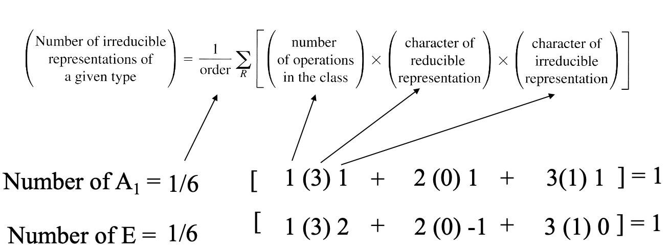
At first glance it looks as though we had found only two of the three expected irreducible representations. However, we need to consider that the symmetry type E is double-degenerate, so it counts like two irreducible representations. Consequently, two of the three ligand orbitals belong to this symmetry type, and are double-degenerated. The third one has the symmetry type A₁.

Symmetry types of Central Atom Orbitals of NH₃

Next, we need to determine the symmetry type of the central atom orbitals. A quick look into the character table can tell us that (Fig. 3.2.26).

Figure 3.2.26 Character table for C_3v and the symmetry types of the N valence orbitals.

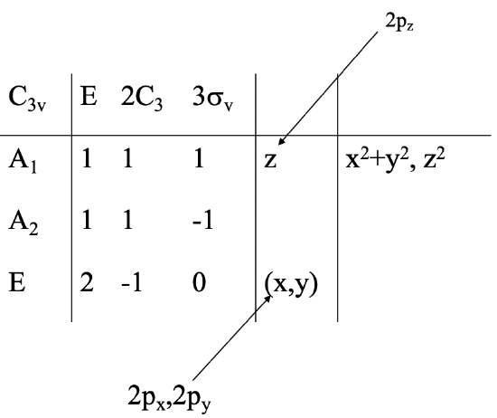
The 2s orbital must have the totally symmetric symmetry type, thus it must have the symmetry type A₁. The 2p_x and the 2p_y orbitals are found in the row for the symmetry type E. They are double-degenerated as one can see from the fact that the letters x and y are in parentheses. The 2p_z orbital has A₁ symmetry, because the letter z can be found the row of the symmetry type A₁.

Combination of the AOs and LGOs of NH₃ to form MOs

Now we must again combine central atom AOs and LGOs of the same symmetry type to form molecular orbitals. The molecular orbitals will have the same symmetry type than the AOs and LGOs from which they have been made. The number of MOs of a specific symmetry type must be equal to the sum of the LGOs and AOs that have the same symmetry type. When an orbital does not find a partner orbital of the same symmetry type, then it is non-bonding.

Let us apply these ideas to the ammonia molecule. We saw that there were two AOs that had the symmetry type A₁, namely the 2s and the 2p_z orbitals. There was also an LGO with A₁ symmetry. We can therefore combine these three orbitals to form molecular orbitals. They also must have the symmetry type a₁.

Figure 3.2.27 Combination of the AOs and LGOs of the A₁ symmetry type in NH₃

Next, let us think about orbitals of the symmetry type A₂. No AO and no LGO has this symmetry type. Therefore, there are also no MOs of this symmetry type. For the symmetry type E we find that there are two AOs, namely the 2p_x and the 2p_y orbital and two LGOs that have this symmetry type. This means that these two orbitals can be combined to form four MOs of the E symmetry type (Fig. 3.2.28).

Figure 3.2.28 Combination of the AOs and LGOs of the E symmetry type

The MO Diagram of NH₃

Now we can construct the MO diagram of NH₃ (Fig. 3.2.29).

Figure 3.2.29 MO diagram of NH₃

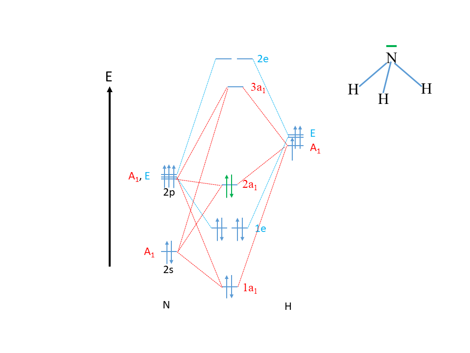
First, we draw the energy axis and indicate the atoms N and H on the left and the right side of the diagram. In the next step we draw the atomic orbitals for the N atom and indicate the symmetry type. The 2s orbital must be drawn below the 2p orbitals to indicate their lower energy.

Then, we can draw the ligand group orbitals on the right side of the diagram and indicate the the symmetry. We can draw the A₁-type LGO somewhat below the E-type orbitals because it has a somewhat lower energy, but this is optional. We know that three MOs with a₁ symmetry must form. When three MOs form then we can estimate that one will be a low-energy bonding one, one will be a high-energy anti-bonding one, and the third one will be an approximately non-bonding one of intermediate energy. Therefore, we will draw the bonding 1a₁-orbital below the 2s orbital, and the anti-bonding 3a₁ orbital above the A₁-type LGO, and the 2a₁ orbital about half-way in between. We also label the MOs according to the energy with the labels 1a₁, 2a₁, and 3a₁, respectively. Lastly, we interconnect the AO and LGOs of the symmetry type A₁ with the a₁-type MOs through dotted lines. They are shown in red (Fig. 3.2.29).

Then, we draw the four E-type MOs. Because the symmetry type E implies that the orbitals are double-degenerate, we know that there must be two double-degenerate bonding MOs and two double-degenerate anti-bonding MOs of the symmetry type E. A valuable property of group theory is that double-degeneracy in symmetry also implies double-degeneracy in energy, and this means that we know that the two bonding MOs have the same energy, and the anti-bonding MOs also have the same energy. We must also draw them this way into the MO diagram. The bonding pair is labeled 1e and the anti-bonding pair is labeled 2e. We cannot know this for sure based on qualitative inspection, but we can suspect that the two bonding e-type orbitals have an energy in between the 1a₁ and the 2a₁ orbital. The 2a₁ orbiital is higher than the 1e orbital because the former is approximately non-bonding, and the latter is bonding. The 1a₁ orbital is likely lower in energy than the 1e orbital because the 1a₁ orbital has a contribution from the low-energy 2s orbital, while the 1e orbital only has contributions from the energetically higher 2p orbitals. By similar arguments we can explain that the 2e orbital has a somewhat higher energy than the 3a₁.

Now we still need to fill the electrons into the orbitals. The N atom has five valence electrons, two being in the 2s, and three being in the 2p orbitals. The three LGOs of H contain one electron each. This gives overall 5+3=8 electrons that we need to fill into the MOs according to energy. That fills the 1a₁ orbital first, then the two 1e₁ orbitals, and finally the 2a₁ orbital. This makes the 2a₁ orbital the HOMO in the molecule, and the 3a₁ the LUMO in the molecule.

We can also make again a comparison of the MO and the Lewis-dot picture of the covalent bonding. We can view the non-bonding HOMO the equivalent of the electron-lone pair at N. There are six electrons in bonding MOs which is the equivalent of the six bonding electrons in the Lewis-dot structure. However, in the MO diagram we can see that the six electrons are not equivalent in energy. We are not able to see that in the Lewis-dot structure. Again, we can conclude that the MO diagram gives us more information about the bonding, which comes at the expense of the increased effort to construct an MO diagram.