3.1: Introduction into Molecular Orbital Theory

Covalent Bonding: Molecular Orbital Theory

Now that we have thoroughly studied symmetry, we can next apply symmetry to molecular orbital theory. Molecular orbital theory is a bonding theory that has been developed to explain covalent bonding, but as we will see in a bit, it can also make statements about ionic bonding. We will see that the application of symmetry to molecular orbital theory will greatly help us to understand molecular orbitals, in particular for more complex molecules. Before we apply symmetry to molecular orbital theory, however, let us briefly review the principles of molecular orbital theory.

Like all theories it is based on a few basic assumptions, also called axioms. The first assumption is the Born-Oppenheimer approximation. It says that the position of the nuclei are nearly fixed relative to electron motion (Fig. 3.1.1).

Figure 3.1.1 The Born-Oppenheimer approximation

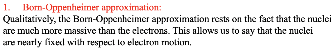
This is a good approximation because the nuclei are much more massive than the electrons. The second axiom is that molecular orbitals can be described as a linear combination of atomic orbitals (Fig. 3.1.2). Linear combination means a vectorial addition or subtraction.

Figure 3.1.2 The second axiom of molecular orbital theory.

Since orbitals are so-called vector functions they can be added and subtracted like vectors. Any orbital is a wave function that has a specific amplitude at a particular point in space. A point in space is defined by a vector that points from the origin to that point in space. Therefore, there is an amplitude associated with each vector that is associated with the wave function. In mathematical form we can say that a molecular orbital Ψ_ab = N (c_aΨ_a ± c_bΨ_b), whereby Ψ_a is the atomic orbital a of atom a, and Ψ_b is the atomic orbital b of atom b. The coefficients c_a and c_b determine how much the specific atomic orbitals a and b contribute to the molecular orbitals. The larger the coefficient, the greater the contribution of the particular atomic orbital to the molecular orbital.

N is the so-called normalization factor. The normalization factor has a value so that the probability to find the electron anywhere within the molecular orbital is 100%. Like in atomic orbitals, the square of the wave function for a molecular orbital reflects the probability to find the electron at a particular position, when we view the electron as a particle. Therefore, the integral of the square of the wave function over space must be 1, and the normalization factor is chosen so that it is 1. The number of orbitals that can be combined to molecular orbitals is not restricted to two. Also three, four or more orbitals can be combined. The number of molecular orbitals that results from a combination of atomic orbitals is always the sum of the atomic orbitals. So when two atomic orbitals are combined, two molecular orbitals must result, when three atomic orbitals are combined, three molecular orbitals must result, and so forth.

How can we qualitatively understand that the vectorial addition of atomic orbitals to form molecular orbitals explains covalent bonding? The nature of the covalent bond is that electrons are being shared between and that the bonds are directional. If we bring two atomic orbitals closer together they will start to interfere.

For example, two 1s orbitals of two hydrogen atoms will start to interfere as we bring the two atoms closer together. If that interference is constructive then the amplitudes of the two wave functions will add up and result in an increased amplitude between the atoms. This addition of amplitudes can be mathematically described by the vectorial addition of the atomic orbital amplitudes. An increased amplitude is associated with an increased electron density between the atoms. Because this electron density is located in between the atoms it can be interpreted as “shared” electron density explaining a directional, covalent bond. The molecular orbital can be called a bonding molecular orbital (Fig. 3.1.3).

Figure 3.1.3 Bonding molecular orbital of the 2s orbitals of two hydrogen atoms (Attribution: www.falstad.com/qmmo/)

However, we must also consider that negative interference can occur which can be described by vectorial subtraction of the amplitudes of the atomic orbitals. In this case the electron-density is depleted in between the atoms, and there is actually a node in between the atoms where the wave function of the molecular orbital changes its algebraic sign. This molecular orbital can be called an anti-bonding molecular orbital (Fig. 3.1.4).

Figure 3.1.3 Anti-bonding molecular orbital of the 2s orbitals of two hydrogen atoms (Attribution: www.falstad.com/qmmo/)

The anti-bonding orbital has a higher energy than the bonding molecular orbital. This can be qualitatively understood from the fact that the energy of wave functions increases with the number of nodes. We have seen this principle before when we discussed atomic theory, and now we meet it again in molecular orbital theory. If a covalent bond forms will depend how many the electrons will be in the bonding or anti-bonding orbitals.

Electrons tend to occupy the lower energy states first, and therefore bonding orbitals will be filled first. However, the Pauli principle holds for molecular orbitals as it holds for atomic orbitals, and therefore we cannot fill more than two electrons in one molecular orbital. Once the bonding molecular orbital is filled, we must start to fill the anti-bonding orbital.

Figure 3.1.5 Equation for the calculation of bond order

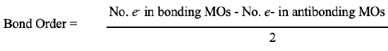
We can define a bond order in the molecule by subtracting the number of electrons in anti-bonding orbitals from the number of bonding orbitals, and divide the resulting number by two (Fig. 3.1.5).

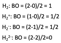
If we stick to our example, the two H atoms, then we have two electrons overall to consider. We can fill both electrons into the bonding molecular orbital, and the anti-bonding molecular orbital remains empty. This gives a bond order of (2-0)/2=1. Therefore, we can say that one covalent bond has formed between the H atoms, have we have produced an H₂ molecule.

Generally we can say that a molecule would expected to be stable when the bond order is larger than 0. That would mean that an H₂⁺ molecular ion should be stable because its bond order would be (1-0)/2=½. The H₂⁺ ion has only one electron which would be in the bonding orbital. However, this bond order is smaller than that of H₂, and thus it should be less stable than H₂. This is in accordance with experimental observations. Also an H₂^- ion should be stable. In this case, one of the three overall electrons would be in the anti-bonding orbital. The bond order would be (2-1)/2=1/2. An H₂^2- anion, however would be expected to be unstable because there would be two electrons in bonding molecular orbitals, and two in anti-bonding ones, resulting in a bond order of (2-2)/2=0 (Fig. 3.1.6).

Figure 3.1.6 Bond order calculations for H₂, H₂⁺, H₂^- and H₂^2-

Molecular Orbital Diagram of H₂

The covalent bonding in a molecule can be described by a molecular orbital diagram. Let us briefly review the principles of its construction for the example of the H₂ molecule (Fig. 3.1.7).

Figure 3.1.7 Molecular orbital diagram of H₂

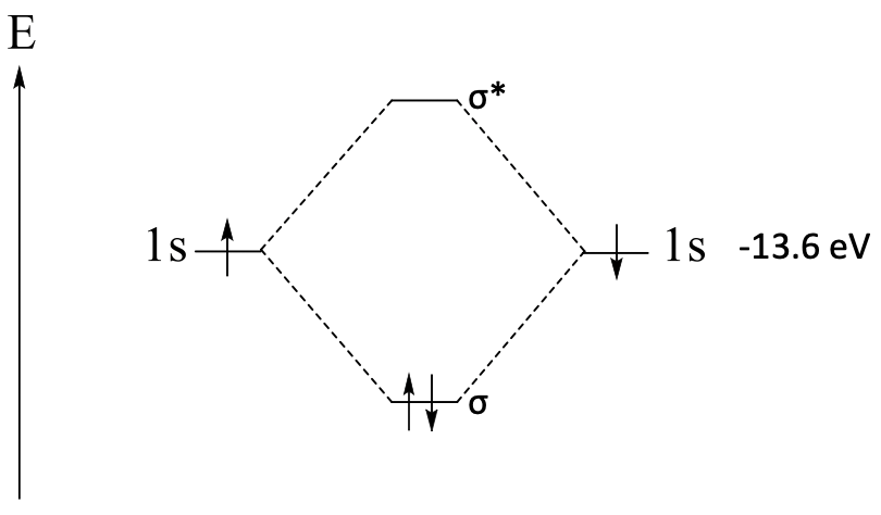
Firstly, we write an arrow to the left. It indicates the relative energies of the orbitals, and is labeled with an E, standing for energy.

Next, we indicate the two 1s atomic orbitals by two horizontal lines, and give them appropriate labels. The lines must be at the same energy levels in the diagram, as both 1s orbitals have the same energy. If you know the exact energy of the orbitals you can write the exact energy next to the orbital name. In the case of the 1s orbitals this would be -13.6 eV.

Next we write the two molecular orbitals as horizontal lines at the appropriate energy levels into the middle of the diagram. The bonding orbital must have a lower energy than the atomic orbitals, and the anti-bonding orbital must have a higher energy. The energy difference between the molecular orbitals and the atomic orbitals must be approximately the same. Typically, the bonding orbital is slightly less bonding than the anti-bonding orbital is anti-bonding. When constructing qualitative molecular orbital diagrams, we do not know the exact energy values for the molecular orbitals, but we can estimate the relative energies of the orbitals according to the arguments just discussed. In the case of the H₂ molecule the two 1s atomic orbitals overlap in σ-fashion, we can therefore denote the molecular orbitals with a σ symbol which we can write next to the lines for the orbitals. The anti-bonding MO gets a * in addition to indicate its anti-bonding nature. We connect the molecular orbitals with atomic orbitals by dotted lines to indicate that the molecular orbitals have been constructed from the 1s atomic orbitals.

In the last step, we fill the electrons into the atomic and molecular orbitals. Each hydrogen has one 1s electron, and we write the electrons as arrows in the 1s orbitals. One electron should be spin up and the other one spin down, because the electrons must have paired spins in the molecular orbital, and spin-reversal is quantum-mechanically forbidden. Lastly, we fill the two electrons into the molecular orbitals according to energy. This means we must write them with with paired spins into the bonding molecular orbital. Now our molecular orbital diagram is complete.

Factors Influencing the Degree of the Covalent Interaction

Now let us refine our understanding of molecular orbitals and molecular orbitals diagrams. Not all atomic orbitals can be combined to form molecular orbitals, and the degree of covalent interaction between two atomic orbitals can vary lot. What are the criteria according to which we can decide if covalent interaction between two atomic orbitals is possible, and if so how much? There are three criteria to consider.

The symmetry criterion, the overlap criterion, and the energy criterion. The symmetry criterion says that if there is a combination of atomic orbitals with bonding and the antibonding interactions that do not cancel out then there is a bonding interaction. We will discuss in a moment what this means.

Definition: Symmetry Criterion

If there is a combination of atomic orbitals with bonding and the antibonding interactions that do not cancel out then there is a bonding interaction.

The overlap criterion states that the better the atomic orbitals (of appropriate symmetry!) overlap the stronger the covalent interaction.

Definition: Overlap Criterion

The better the atomic orbitals (of appropriate symmetry!) overlap the stronger the covalent interaction.

The energy criterion states that the closer the orbitals are in energy the more covalent interaction between them.

Definition: Energy Criterion

The closer the atomic orbitals in energy the stronger the covalent interaction.

The Overlap Criterion

Let us now look at each criterion in more detail. Let us start with the one we can probably most easily understand, the overlap criterion. The greater the overlap the greater the covalent interaction. The overlap can be estimated according to three rules.

Rule 1

The first rule says that the overlap is the greater the smaller the distance between the two orbitals (Fig. 3.1.8).

Figure 3.1.8 Rule 1 for the overlap criterion

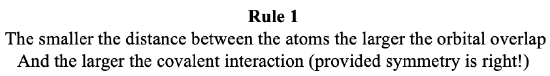
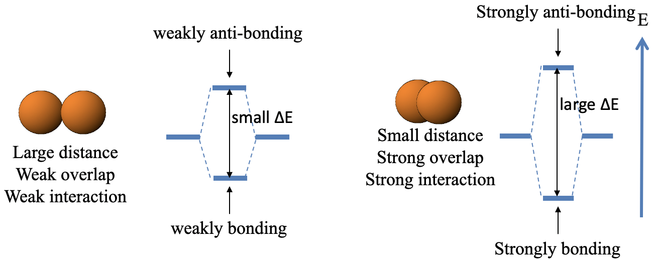
This means that a small distance between the orbital leads to a strongly bonding and a strongly anti-bonding orbital, respectively while a large distance leads to a weakly bonding and a weakly anti-bonding orbital. When the distance is small then there is a large energy difference between the bonding and the anti-bonding molecular orbital, when the distance is large then the energy difference is small (Fig. 3.1.9).

Figure 3.1.9 The effect of the distance between atomic orbitals on the energy difference of the resulting molecular orbitals.

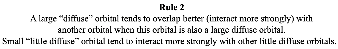
Rule 2

Rule 2 states that a large “diffuse” orbital tends to overlap better (interacts more strongly) with another orbital when this orbital is also a large diffuse orbital. Small “little diffuse” orbital tend to interact more strongly with other little diffuse orbitals. If we combine a large orbital with a small orbital however, then this typically does not lead to good overlap and thus weak interaction (Fig. 3.1.10).

Figure 3.1.10 Rule 2 for the overlap criterion

We can qualitatively understand this by looking at the image below (Fig. 3.1.11).

Figure 3.1.11 Relationships between orbital size and covalent interactions.

Only a small volume fraction of the large orbital can overlap with the small orbital due to the small size of the small orbital. Due that small overlap the bonding orbital is only weakly bonding, and the anti-bonding is only weakly anti-bonding. The energy difference between the bonding and the anti-bonding orbital is small. In the other two cases, the bonding orbitals tend to be strongly bonding, and the anti-bonding ones strongly anti-bonding. The energy differences between the orbitals tend to be large.

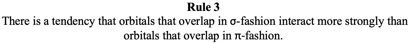
Rule 3

Rule 3 says that that orbitals that overlap in σ-fashion tend to interact more strongly than orbitals that overlap in π-fashion (Fig. 3.1.12).

Figure 3.1.12 Rule 3 for the overlap criterion

One can see easily from the image below that two p orbitals that have the same distance d from each other overlap much more when they overlap in σ-fashion compared to π-fashion (Fig. 3.1.13).

Figure 3.1.13 Visual representation of orbitals overlapping in σ-fashion vs orbitals overlapping in π-fashion

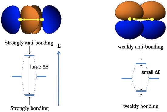
This is because in the first case they point toward each other, and the orbital overlap is on the bond axis, while in the latter case they are oriented parallel to each other, and the orbital overlap is above and below the bond axis. This implies that the σ-overlap leads to more bonding and anti-bonding orbitals with a larger energy gap between them compared to the π-overlap.

The Energy Criterion

The energy criterion states that the covalent interaction is the larger the smaller the energy difference between the atomic orbitals. We can understand this qualitatively when considering that orbitals are waves, and waves of similar energy interfere more significantly with each other than waves with different energies. Just imagine two waves with very different wavelengths associated with very different energies. Would they interfere effectively? No, they wouldn’t. Rather, two waves with very similar wavelengths would interfere better. Because greater energy difference means less interaction, molecular orbitals that result from the interaction of two atomic orbitals with large energy difference are much more similar in shape, size, and location compared to molecular orbitals that result from atomic orbitals with similar energy.

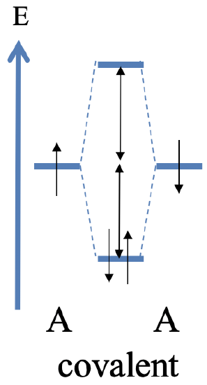
The greatest covalent interaction is expected when the energy between the two orbitals is exactly the same. This is only possible when two, same orbitals A of the two same atoms overlap. In this case we form a perfect covalent bond with electrons exactly equally shared between the orbitals. The maximum of the amplitude of the bonding molecular orbital is exactly in the middle between the two atoms. In the molecular orbital diagram the energy difference between the bonding MO and the AOs is about the same as the energy difference between the anti-bonding MO and the AOs. Assuming that each atomic orbital is filled with one electron the two electrons are in the bonding molecular orbital where they are equally shared between the atoms (Fig. 3.1.14)

Figure 3.1.14 Covalent interaction occurring when the energy between the two atomic orbitals is exactly the same

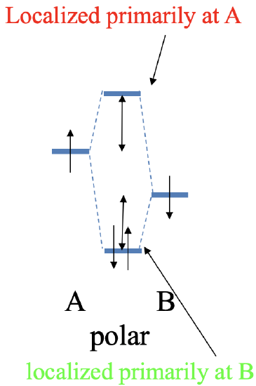
Now let us make the energy of the two atomic orbitals somewhat different. Because they are different we denote the atomic orbitals A and B now, whereby we choose the energy of orbital A to be somewhat higher than that of orbital B. Overlap between the atomic orbital still produces covalent interaction yielding a bonding and an anti-bonding molecular orbital. However, the energy difference of the molecular orbitals to the two atomic orbitals is no longer the same. The anti-bonding MO is now closer to the AO with the higher energy, and the bonding MO is now closer in energy to the AO with the lower energy. This has another consequence. The bonding molecular orbital is now localized primarily at atom B, and the anti-bonding orbital is located primarily at atom A. If we again assume that each AO contributed one electron to the covalent bond, then the two electrons will be in the bonding MO. Because the bonding MO is now primarily localized at atom B, the bonding electrons are primarily localized at atom B. This means they are no longer exactly equally shared, and we have a polar, covalent bond which his polarized toward atom B (Fig. 3.1.15).

Figure 3.1.15 An example of covalent interaction occurring when the energy between the two atomic orbitals is somewhat different

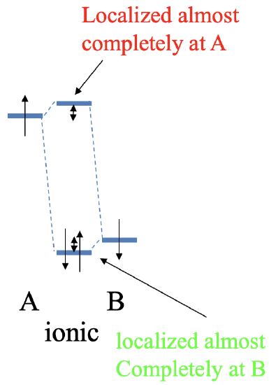
Now let us make the energy difference between the two atomic orbitals of the atoms A and B very large (Fig. 3.1.16). In this case, the bonding MO is energetically very close to the AO of atom B, and is localized almost exclusively at atom B. Actually, the bonding MO closely resembles the AO of atom B in shape, size and localization. In other words, the AO of B has hardly changed due to the very weak covalent interaction resulting from the large energy difference between the atomic orbitals. Vice versa, the anti-bonding orbital is energetically very close to the AO of atom A, and is localized almost completely at atom A. The anti-bonding MO is very close to the AO in shape, size, and location. Due to the weak covalent interaction, there is almost no change to the atomic orbital of A. Assuming that each atomic orbital contributes two electrons, the bonding orbital will be filled. The two electrons will be almost exclusively located at atom B. This means that we have effectively transferred one electron from atom A to atom B in a redox process, and have produced an ionic bond. Atom A has now effectively a 1+ charge, and atom B has a 1- charge. This shows that molecular orbital theory, although designed for covalent bonding, can also make statements about ionic bonding. We can also see that a 100% ionic bond is not possible. To achieve 100% iconicity the energy difference between the two atomic orbitals would need to be infinitely large. This is practically impossible. However, a 100% covalent bond is possible because two electrons can be exactly equally shared between two atoms when the energy of the atomic orbitals is exactly zero.

Figure 3.1.16 Covalent interaction occurring when the energy difference between two atomic orbitals is very large.

Another conclusion that we can draw is that bonding electrons are located at the atom with the atomic orbital of lower energy, and anti-bonding electrons are located at the atoms with the atomic orbital of higher energy. Orbital energy is correlated with electronegativity. For orbitals of the same type and the same elements, orbitals with higher electronegativity have lower energy. For example, a 2s orbital of fluorine has a lower energy than a 2s orbital of oxygen because the electronegativity of fluorine is higher. Bonding electrons are therefore located primarily at the more electronegative atom, while anti-bonding electrons are located primarily at the less electronegative atom (Fig. 3.1.7). When there are enough anti-bonding orbitals occupied it is possible that the overall polarity in the molecule is such that the dipole moment points toward the more electro-positive atom. An example is carbon monoxide which is slightly polarized toward the carbon atom. We will discuss the MO diagram of the carbon monoxide in detail later.

Figure 3.1.17 Relationship between orbital energy and electronegativity

The Symmetry Criterion

Lastly, let us look at the symmetry criterion. The symmetry criterion tells us if a covalent interaction between orbitals is possible based on the relative orientation of the orbitals. Only if bonding and anti-bonding interactions do not cancel out, a bonding interaction is possible, and we can construct molecular orbitals from atomic orbitals. Bonding and anti-bonding interactions cancel out when positive and negative interferences due to orbital overlap are exactly equal. This can be determined by inspection of orbital overlap.

For example, let us look at the orbital overlap between the 1s orbitals of hydrogen and the 2p_z orbital of oxygen in the water molecule (Fig. 3.1.18).

Figure 3.1.18 The orbital overlap between the 1s orbitals of hydrogen and the 2p_z orbital of oxygen in the water molecule

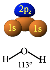
In the water molecule the orbitals are oriented to each other in a specific way because of the bent structure of the water molecule. Due to the bent structure of the water molecule the 1s orbitals overlap differently with the two lobes of the 2p_z molecule. The lobe that points downward overlaps more strongly than the lobe that points upward. The two lobes must have different algebraic sign. Now we choose the algebraic sings of 1s orbitals so that bonding is maximized. This means that we choose the algebraic signs so that they are the same as the those of the lobe that points downward. We can see that now the overlap of the 1s with the 2p_z orbital produces more positive than negative interferences. The blue lobe is further away from the 1s orbitals than the orange lobe and thus positive and negative interferences do not cancel out. This is equivalent to saying that bonding and anti-bonding interactions do not cancel out. Therefore, the symmetry is “right”, we can construct molecular orbitals from this combination of atomic orbitals.

Can the 2p_x orbital of oxygen also combined with the 1s orbitals of the hydrogen atom to form molecular orbitals? The 2p_x orbital is oriented differently relative to the 1s orbitals in the H₂O molecule (Fig. 2.1.19).

Figure 3.1.19 The orbital overlap between the 1s orbitals of hydrogen and the 2p_x orbital of oxygen in the water molecule shown in two different orientations

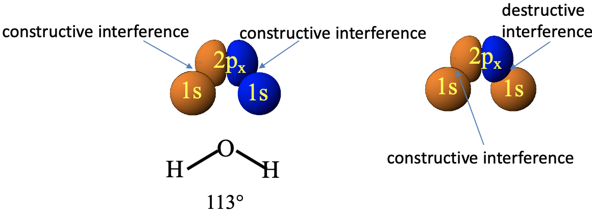
In this case, we must choose the algebraic signs of the two 1s orbitals to be different so that bonding interactions are possible. The bonding and the antibonding interactions only do not cancel out if the left 1s orbital has the same algebraic sign as the left lobe of the 2p_x orbital and the right 1s orbital has the same algebraic sign as the right lobe of the 2p_x orbital. If, for instance, we chose both 1s orbitals to be orange, then the bonding interactions between the left lobe and the left 1s orbital would be canceled out by the equally strong anti-bonding interactions between the right lobe and the right 1s orbital. Overall, we see however, that if we select the color (meaning algebraic sign) of the 1s orbitals appropriately then the symmetry is “right” and we can create molecular orbitals from the atomic orbitals.

What about the combination of the 2s of the oxygen with the 1s orbitals of the hydrogens (Fig. 3.1.20)?

Figure 3.1.20 The orbital overlap between the 1s orbitals of hydrogen and the 2s orbital of oxygen in the water molecule

We can see that is very easy to construct a combination in which there are bonding interactions. If we choose the algebraic sign of all atoms to be the same, then certainly bonding and anti-bonding interactions do not cancel out. The symmetry is “right”, and the construction of atomic orbitals from molecular orbitals is possible.

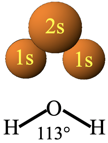
What about the interactions between the 1s orbitals and the 2p_y orbital (Fig. 3.1.21)?

Figure 3.1.21 The orbital overlap between the 1s orbitals of hydrogen and the 2p_y orbital of oxygen in the water molecule shown in two different orientations

In this case, the two 1s orbitals are in the paper plane, and the 2p_y orbital stands perpendicular to it. That makes a 1s orbital to overlap equally with both lobes of the 2p_y orbital. Because the two lobes of a 2p_y orbital must have different algebraic sign, the constructive and the destructive interferences will cancel out, no matter how we chose the algebraic signs of our 1s orbitals. That means there is no possibility to create orbital overlap in which bonding an anti-bonding interactions do not cancel out. Therefore, we cannot produce molecular orbitals from a combination of 1s and 2p_y orbitals. The 2p_y must remain non-bonding. You may be able to see the cancelation of the bonding and antibonding orbital overlap better if you choose your coordination system differently. Let us have the y-axis point up, and the x-axis point right (Fig. 3.1.21, bottom). Now we look at the H₂O molecule from the bird perspective, and the 2p_y orbital is oriented vertically. The 1s orbitals are still on the x-axis. You can see the overlap between the 1s orbitals and the 2p_y orbital more clearly now. No matter how we choose the algebraic sign of our orbitals, the bonding and the anti-bonding interactions cancel out.

We have seen thus far that is is possible to decide about “right” and “wrong” symmetries by inspection, but we have noticed that this is not trivial. Generally, the more complex a molecule gets the more difficult it is to decide about “right” and “wrong” symmetry. As we will see in the following, group theory can greatly help us decide about “right” and “wrong” symmetry. It provides a formal pathway to unambiguously make such a decision.

---

Dr. Kai Landskron (Lehigh University). If you like this textbook, please consider to make a donation to support the author's research at Lehigh University: Click Here to Donate.