11.2: Quantum Numbers of Multielectron Atoms

Note

The quantum numbers of atoms (and ions) correspond to quantized energy states, called microstates, that depend on the electron configuration. Electrons within a subshell or orbital can adopt different configurations of their electrons, with different individual quantum numbers. These different electron configurations are microstates, and they can be grouped into terms and ordered according to their relative energies. Since electronic transitions occur between terms of different energies, knowledge of the terms for a given atom or ion can aid in the interpretation of electronic spectra.

Introduction

Transition metal ions can give rise to a spectrum of beautifully colored colored complexes. The colors are often caused by absorption of visible light due to electronic transitions involving metal d-orbitals. These electronic transitions are not only attractive to the eye, they are useful spectroscopic signals because the transitions occur between quantized electronic energy states, called microstates. Spectroscopy, coupled with knowledge of the possible microstates and their energies can yield clues about molecular structure.

To learn what a microstate is, let's use the simple example of a carbon atom with a \(1s^2 2s^2 2p^2\) electron configuration. The \(s\) subshell is full, and there is only one way to put two electrons into an \(s\) subshell. Both electrons must occupy the orbital having \(m_l=0\), and each must have opposite spins, (\(m_s =+\frac{1}{2}\)), and (\(m_s =-\frac{1}{2}\)). On the other hand, the \(p\) subshell of carbon has two electrons that can occupy any of three orbitals (Figure \(\PageIndex{1}\)). This leaves room for different orientations of the electrons within the \(p\) subshell. Each different electron configuration is a microstate, and each has an energy that can be distinguished using electronic spectroscopy (UV-vis for example). In the case of a carbon atom with a two \(p\) electrons, there are 15 different possible microstates, as illustrated in Figure \(\PageIndex{1}\).

Figure \(\PageIndex{1}\): Fifteen possible microstates for two electrons in a \(p\) subshell. These microstates are organized according to their total spin (\(M_s\)) and total magnetic (\(M_l\)) quantum numbers. Arrows pointing upward represent electrons with \(m_s = +\frac{1}{2}\), and those pointing downward represnt \(m_s = -\frac{1}{2}\). Each horizontal line represents a \(p\) orbital, and \(m_l\) values are indicated under each orbital. (CC-BY-NC; Kathryn Haas)

Just as individual electrons have quantum numbers (\(n, l, m_l, m_s\)), the electronic states of atoms have quantum numbers (\(L, M_l, M_s, S, J\)). Each individual microstate in Figure \(\PageIndex{1}\) can be described by quantum numbers \(M_l\) and \( M_s\). The values of total angular momentum (\(L\)), and total intrinsic spin (\(S\)) arise from sets of microstates, and are related to quantum numbers \(M_l\) and \(M_s\) for individual microstates. The relative energies of the terms for 3d metals and other light atoms can be predicted (roughly) by Hund's Rules, according to values of S and L. These atomic quantum numbers and Hund's rules are described below.

A closer look at electronic spectra

Let us take a closer look at optical absorption spectra, also called electronic spectra, of coordination compounds. We have previously argued that ligand field theory can predict and explain the electronic spectra. However, ligand field theory (LFT) is sufficient to explain the spectra in only a few cases. For example the \(\ce{[Ni(H2O)6]^2+}\) ion is an octahedral \(d^8\)-complex ion. According to LFT, the metal \(d\)-orbitals in an octahedral field are the \(t_{2g}\) and the \(e_g\)–orbitals (Figure \(\PageIndex{2}\)). Six electrons are in the \(t_{2g}\) orbitals, and two electrons are in the \(e_{g}\) orbitals (Figure \(\PageIndex{2}\)). Ligand field theory (LFT) would predict that there is one electron transition possible, namely the promotion of an electron from a \(t_{2g}\) into an \(e_{g}\) orbital. This process would be triggered by the absorption of light whereby the wavelength of the light would depend on the \(\Delta_o\) between the \(t_{2g}\) and the \(e_{g}\) orbitals. Overall, this should lead to a single absorption band in the absorption spectrum of the complex. We can check this prediction by experimentally recording the absorption spectrum of the complex (Figure \(\PageIndex{2}\)).

Figure \(\PageIndex{2}\). Electron transition according to LFT and actual absorption spectrum of the \(\ce{[Ni(H2O)6]^2+}\) complex ion. Attribution: E.R. Schofield.

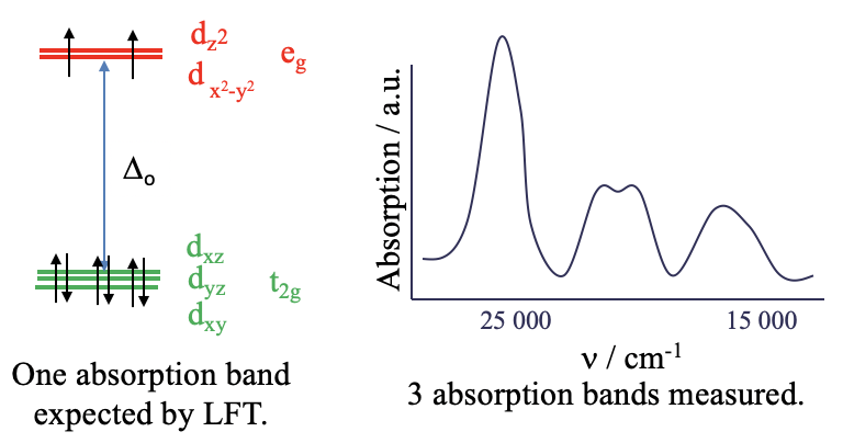
What we find is that the absorption spectrum is far more complex than expected. Instead of just a single absorption band there are multiple ones. Obviously, LFT is unable to explain this spectrum. The question is: why? The answer is: LFT assumes that there are no electron-electron interactions. However, in reality there is repulsion between electron in d-orbitals and this has an effect on their energy. And, electrons within the d-subshell, for example, repel each other to different extents depending on the relative orientations of their orbitals in space.

To illustrate how electrons in different orbitals might have different interactions, let's consider the case of a \(d^2\) excited state in an octahedral ligand field (Figure \(\PageIndex{3}\)).

Figure \(\PageIndex{3}\): Two microstates with different energies for a \(d^2\) ion in an octahedral ligand field. Electron configurations of two different microstates are shown on the top, and the orbitals associated with each shown underneath each configuration. Left: An excited microstate with one electron in the \(d_{xy}\) orbital (shown in green) and one electron in the \(d_{z^2}\) (shown in red). Right: An excited microstate with one electron in the \(d_{xz}\) orbital (shown in green) and one electron in the \(d_{z^2}\) (shown in red).

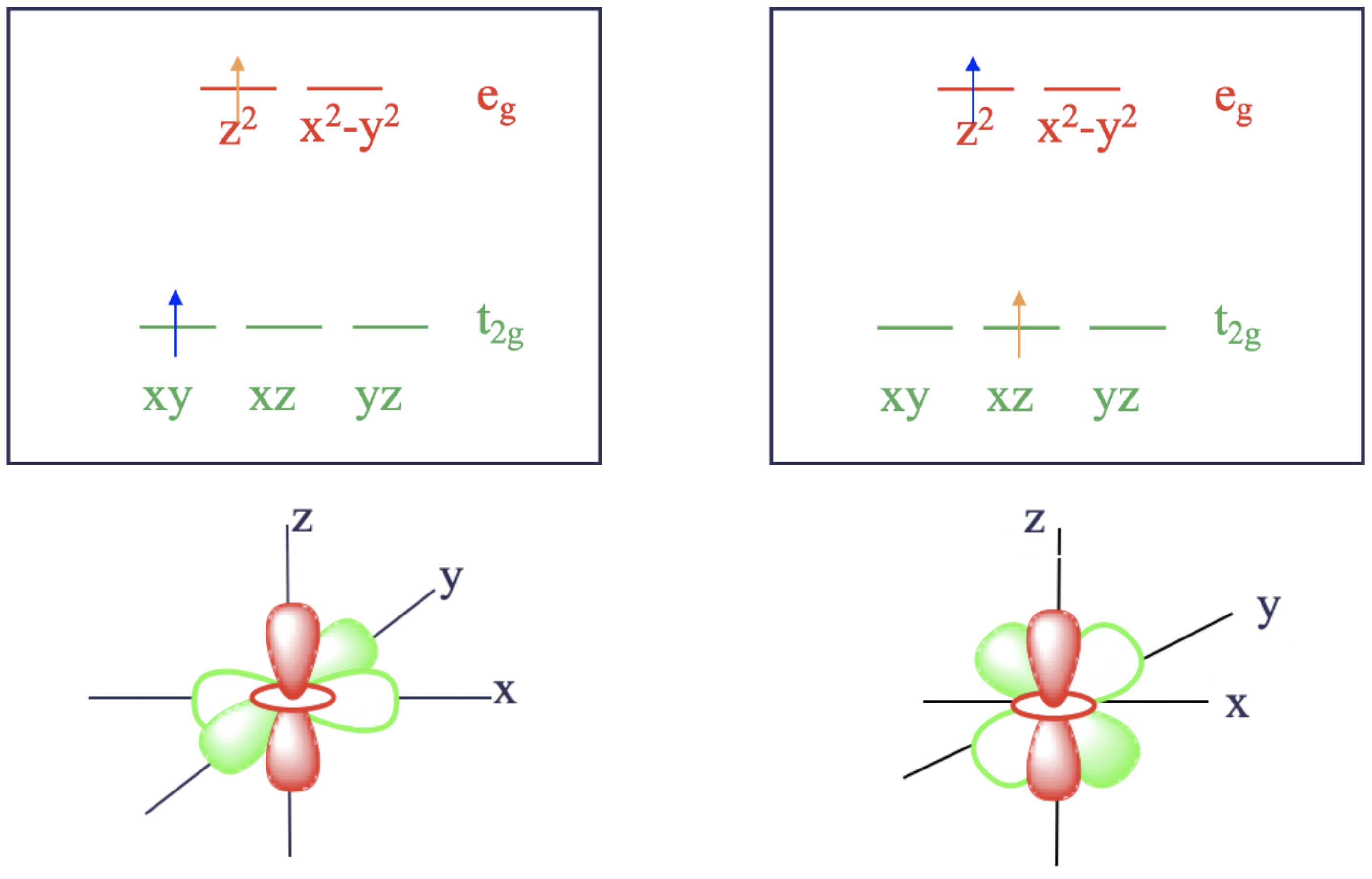
According to LFT, both electrons would be in the \(t_{2g}\) orbitals in the ground state. For instance, they could be in the microstate where one electron is in \(d_{xy}\), and the other is in the \(d_{xz}\) orbital (not pictured). This configuration is called a microstate of a state because there are other combinations of orbitals possible. For example, the ground state would also be realized by a microstate in which the electrons were in the \(d_{xz}\) and the \(d_{yz}\) orbitals. Upon absorption of light, the electron in the \(d_{xy}\) orbital could be excited into one of the higher-energy \(e_{g}\) orbitals. That excited electron could occupy either the \(d_{z^2}\) or the \(d_{x^2-y^2}\) orbitals. Those two possibilities reflect two different microstates associated with the excited state. For a moment, let's assume that the excited electron goes into the \(d_{z^2}\) orbital. In this microstate one electron would be in the \(d_{xz}\) orbital and the other one in the \(d_{z^2}\) orbital (Figure \(\PageIndex{3}\), right). There is another possibility for how to excite an electron from the ground state. We could assume that instead of the \(d_{xy}\) electron being promoted, the \(d_{xz}\) electron gets promoted. In this case, we would realize a microstate in which one electron in the \(d_{xy}\) orbital and the other one in the \(d_{z^2}\) orbital (Figure \(\PageIndex{3}\), left).

Now let us compare the two cases shown in Figure \(\PageIndex{3}\). Ligand field theory would argue that both excited microstates have the same energy. However, in fact they do not. Why? It is because the electrons in the first excited microstate interact differently than those of the second excited microstate. This difference becomes plausible when considering the orbital shapes and orientations (Figure \(\PageIndex{3}\), bottom). The \(d_{xz}\) orbital has electron density on the z-axis, while the \(d_{xy}\) orbital is perpendicular to \(d_{z^2}\). The different relative orientations of \(d_{xy}\) and \(d_{xz}\) with respect to \(d_{z^2}\) cause electrons in the \(d_{z^2}\) orbital to interact differently with an electron in a \(d_{xy}\) than in a \(d_{xz}\). As a result, the two excited microstates do not have the same energy. In other words, to achieve either of these different excited microstates from the ground state, we need different amounts of energy. Thus, the complex would absorb light with different energies (or wavelengths). This is in contrast to what LFT predicts.

If LFT cannot predict the number of electronic transitions, then how can we correctly predict how many absorption bands we get? The answer is, we must find all possible microstates for the \(d^2\) electron configuration and group together those with the same energy. A group of microstates with the same energy is called a term. The number of electron transitions can then be predicted from the number of terms.

Quantum Numbers

The table below summarizes the quantum numbers of atoms (individual microstates and sets of microstates). You may wish to review the quantum numbers for individual electrons and then refer to this table as you read this and the next sections. Recall the meanings of the quantum numbers for individual electrons (\(n, l, m_l, m_s\) that were described in a previous section (Section 2.2.2).

Symbol	Name	Allowed Range	Comment
\(L\)	Total Orbital Angular Momentum	\(|l_1 + l_2 | , |l_1 + l_2 ‐ 1| , \ldots, |l_1 ‐ l_2 |\)	Total orbital angular momentum of a collection of microstates, designated as S, P, D, F..etc
\(S\)	Total Intrinsic Spin	\(|{m_s}_1 + {m_s}_2 |, |{m_s}_1 +{m_s}_2 ‐ 1| , ... ,| {m_s}_1 ‐ {m_s}_2 |\)	Total spin of a collection of microstates
\(M_l\)	Magnetic Quantum Number	\( L, L-1, L-2, ..., -L\)	Direction of total angular momentum for an individual microstate
\(M_s\)	Spin Magnetic Quantum Number	\(S, S-1, S-2, ...-S \)	Total spin of electrons for an individual microstate
\(J\)	Total Angular Momentum	\(L+S,..., | L-S |\)	Total angular momentum

Quantum Numbers S and L for sets of microstates

The quantum numbers \(S\) and \(L\) represent sets of microstates. Once these values are found, they can be ordered in terms of relative energies, first according to the value of \(S\), then \(L\).

Total Orbital Angular Momentum Quantum Number: L

\(L\) gives the total sum of orbital angular momentum vectors in a multielectron atom. The possible values of \(L\) can be found from the values of \(l\) for individual electrons in the system. For example, in a system with two electrons with values of \(m_{l_1}\) and \(m_{l_2}\), the possible values of \(L\) are:

\[ L = \sum_i^n m_{l_i} = |m_{l_1} + m_{l_2} | , |m_{l_1} + m_{l_2} ‐ 1| , \ldots, |m_{l_1} ‐ m_{l_2} | \]

The absolute value symbols indicate that \(L\) cannot be a negative value. The values of \(L\) correspond to different energy levels for groups of microstates. Microstates with values of \(L=0, 1, 2, 3...\) correspond to symbols \(S, P, D, F...\) respectively. This is analogous to the relationship between the electron quantum number, \(l\), and the \(s, p, d, f..\) orbital subshells. However, the capital letters used for microstates do not indicate orbital or subshell assignments for the electrons.

The Total Intrinsic Spin Quantum Number: \(S\)

The sum total of the spin vectors of all of the electrons is called \(S\). The values of \(S\) are computed from \(m_s\) in a manner very similar to how \(L\) is computed from \(m_l\). Because \(S\) measures the magnitude of a vector, it cannot be negative. For a system with two electrons, each with spin \({m_s}_1\), and \({m_s}_2\), the possible values of \(S\) are given below.

\[S =\sum_i^n {m_s}_i = |{m_s}_1 + {m_s}_2 |, |{m_s}_1 +{m_s}_2 ‐ 1| , ... ,| {m_s}_1 ‐ {m_s}_2 | \label{spin}\]

The possible values of \(S\) fall into a series that depend on whether there are an odd or even number of electrons.

• Odd number of electrons: \(S=\frac{1}{2}, \frac{3}{2}, \frac{5}{2},...\)
• Even number of electrons: \(S = 0, 1, 2, 3,...\)

Example 11.2.1 : Total Orbital Angular Momentum of Carbon

What are the possible \(L\) values for the electrons in the \(1s^2 2s^2 2p^2\) configuration of carbon?

Solution

Both electrons (i.e., the 2p electrons) are \(l = 1\). The possible combinations are 0, 1, and 2 corresponding to symbols S, P, and D, respectively.

Example 11.2.2 : Total Orbital Angular Momentum of Unknown Species

What are the possible \(L\) values for the electrons in the \([Xe]6s^2 4f^1 5d^1\) ?

Solution

We can ignore the electrons in the \([Xe]\) core and the electrons in the \(6s\) block. So all we have to consider is the lone \(f\) electron (\(l=3\)) and the lone \(d\) electron (\(l=2\)).

The two extremes for possible \(L\) values are \(3+2 = 5 \) and \(3 ‐ 2 = 1\).

Thus, possible values of \(L\) for this Xe atom are 5(H), 4(G), 3(F), 2(D), and 1(P).

Example 11.2.5 : The Hydrogen Ground State

Find \(S\) for \(1s^1\).

Solution

\(S\) must be \(\frac{1}{2}\), since that’s the spin of a single electron and there’s only one electron.

Example 11.2.6 : The Beryllium Excited State

Find S for \(1s^2 2s^1 2p^1\).

Solution

\(S = 1, 0\)

Example 11.2.7 : The Carbon Ground State

Find \(S\) for carbon atoms with the \(1s^2 2s^2 2p^2\) electron configuration.

Solution

\(S=1,0\) This is the same as the previous problem. Notice that \(S\) is not affected by which orbitals are occupied by electrons. \(S\) depends only on the number of unpaired electrons. These are usually the electrons in partially-filled subshells (i.e., unpaired electrons in open shells).

Example 11.2.8 : The Nitrogen Ground State

Find \(S\) for nitrogen atoms with the \(1s^2 2s^2 2p^3\) electron configuration.

Solution

\(S\) can be \(S=\frac{3}{2}, \frac{1}{2}\).

Quantum numbers \(M_l\) and \(M_s\) for individual microstates

Once S and L are found, the allowed values of \(M_l\) and \(M_s\) can be calculated.

The Total Magnetic Quantum Number: \(M_l\)

The Total Magnetic Quantum Number \(M_l\) is the total \(z\)-component of all of the relevant electrons’ orbital momentum. While \(L\) describes the total angular momentum in the system, \(M_l\) tells you which direction it is pointing. \(L\) can be assigned to a collection of microstates, but \(M_l\) is unique to a specific microstate in that group. Unlike \(L\), \(M_l\) is allowed to have negative values. The possible values of \(M_l\) are integer values ranging from the largest positive sum to the most negative sum of possible \(m_l\) values:

\[M_l = L, L-1, L-2, ..., -L \]

For the \(p^2\) case, the \(m_l\) values of \(p\) orbitals are \(-1, 0, +1\). The largest value of \(M_l\) would come from a state where both electrons occupy \(m_l=+1\), thus the maximum is \(M_l=L=2\). Likewise, the minimum value of \(M_l\) comes from both electrons occupying \(m_l=-1\) to give \(M_l=-L=-2\). The possible \(M_l\) values for \(p^2\) are the series of integer values \(+2, +1, 0, -1, -2\).

It is worth noting that there are values of \(M_l\) that are forbidden due to the Pauli exclusion principle. For example, the value of \(M_l=+3\) could only come from three electrons occupying the \(m_l=+1\) orbital. That is impossible because more than one electron would possess the same set of electron quantum numbers.

The Total Spin Magnetic Quantum Number: \(M_s\)

\(M_s\) is the sum total of the z-components of the electrons’ inherent spin in an individual microstate. The difference between \(S\) and \(M_s\) is subtle, but important. \(M_s\) indicates the total z-component of the electrons’ spins, while \(S\) indicates the entire resultant vector. It is also distinct from \(M_l\), which is the sum total of the z-component of the orbital angular momentum. \(M_s\) can be computed from \(S\), as shown below. Note that while \(S\) must be positive, \(M_s\) can have negative values.

\[M_s = S, S-1, S-2, ...-S \label{Ms}\]

For the \(p^2\) case, the possible values of \(M_s\) are \(M_s = +1, 0, -1\). The value \(M_s = +1\) comes from the sum of two electrons with spin "up", \(m_s=+\frac{1}{2}\). The value \(M_s = -1\) comes from the sum of two electrons with spin "down", \(m_s=-\frac{1}{2}\). And the value \(M_s = 0\) comes from the sum of one electron with \(m_s=+\frac{1}{2}\) and the other with \(m_s=-\frac{1}{2}\).

There are some values of \(M_s\) that will be forbidden, but not in the case of \(p^2\). However in the case of a \(p^4\), for example, the value \(M_s\)=2 is forbidden because there is no way to put four "up" electrons in three orbitals without violating the Pauli exclusion principle.

Example 11.2.3 : Total Magnetic Quantum Number of the Zirconium Ground State

What are the possible values \(M_l\) of a zirconium atom with the \([Kr] 5s^2 4d^2\) electron configuration?

Solution

Both open-shell electrons (i.e., the 4d electrons) are \(l=2\), so the values are 4, 3, 2, 1, 0, -1, -2, -3, -4.

Example 11.2.4 : Total Spin Magnetic Quantum Number of the Carbon Ground State

What are the \(M_s\) values for \(1s^2 2s^2 2p^2\) ?

Solution

This system is paramagnetic, with two unpaired electrons in the \(2p\) orbital. The three \(p\) orbitals have values of \(m_s=-1,0,1\). The maximum value of \(M_s=+1\) would come from the two electrons occupying \(m_{s_1}=+1\) and \(m_{s_2}=0\). The minimum value, \(M_s=-1\) would come from the two electrons occupying \(m_{s_1}=-1\) and \(m_{s_2}=0\). Thus, the possible values for the total spin magnetic quantum number are \(M_s = 1, 0, ‐1\), where the value of \(M_s=0\) comes from a configuration where, for example, \(m_{s_1}=+1\) and \(m_{s_2}=-1\).

Example 11.2.4 : Total Spin Magnetic Quantum Number of the Nitrogen Ground State

What are the \(M_s\) values for \(1s^2 2s^2 2p^3\) ?

Solution

\(M_s = +\frac{3}{2}, \; +\frac{1}{2}, \; -\frac{1}{2}, \; -\frac{3}{2}\)