
5.4.5: CO₂ (Revisted with Projection Operators)
- Page ID
- 172985
\( \newcommand{\vecs}[1]{\overset { \scriptstyle \rightharpoonup} {\mathbf{#1}} } \)
\( \newcommand{\vecd}[1]{\overset{-\!-\!\rightharpoonup}{\vphantom{a}\smash {#1}}} \)
\( \newcommand{\id}{\mathrm{id}}\) \( \newcommand{\Span}{\mathrm{span}}\)
( \newcommand{\kernel}{\mathrm{null}\,}\) \( \newcommand{\range}{\mathrm{range}\,}\)
\( \newcommand{\RealPart}{\mathrm{Re}}\) \( \newcommand{\ImaginaryPart}{\mathrm{Im}}\)
\( \newcommand{\Argument}{\mathrm{Arg}}\) \( \newcommand{\norm}[1]{\| #1 \|}\)
\( \newcommand{\inner}[2]{\langle #1, #2 \rangle}\)
\( \newcommand{\Span}{\mathrm{span}}\)
\( \newcommand{\id}{\mathrm{id}}\)
\( \newcommand{\Span}{\mathrm{span}}\)
\( \newcommand{\kernel}{\mathrm{null}\,}\)
\( \newcommand{\range}{\mathrm{range}\,}\)
\( \newcommand{\RealPart}{\mathrm{Re}}\)
\( \newcommand{\ImaginaryPart}{\mathrm{Im}}\)
\( \newcommand{\Argument}{\mathrm{Arg}}\)
\( \newcommand{\norm}[1]{\| #1 \|}\)
\( \newcommand{\inner}[2]{\langle #1, #2 \rangle}\)
\( \newcommand{\Span}{\mathrm{span}}\) \( \newcommand{\AA}{\unicode[.8,0]{x212B}}\)
\( \newcommand{\vectorA}[1]{\vec{#1}} % arrow\)
\( \newcommand{\vectorAt}[1]{\vec{\text{#1}}} % arrow\)
\( \newcommand{\vectorB}[1]{\overset { \scriptstyle \rightharpoonup} {\mathbf{#1}} } \)
\( \newcommand{\vectorC}[1]{\textbf{#1}} \)
\( \newcommand{\vectorD}[1]{\overrightarrow{#1}} \)
\( \newcommand{\vectorDt}[1]{\overrightarrow{\text{#1}}} \)
\( \newcommand{\vectE}[1]{\overset{-\!-\!\rightharpoonup}{\vphantom{a}\smash{\mathbf {#1}}}} \)
\( \newcommand{\vecs}[1]{\overset { \scriptstyle \rightharpoonup} {\mathbf{#1}} } \)
\( \newcommand{\vecd}[1]{\overset{-\!-\!\rightharpoonup}{\vphantom{a}\smash {#1}}} \)
\(\newcommand{\avec}{\mathbf a}\) \(\newcommand{\bvec}{\mathbf b}\) \(\newcommand{\cvec}{\mathbf c}\) \(\newcommand{\dvec}{\mathbf d}\) \(\newcommand{\dtil}{\widetilde{\mathbf d}}\) \(\newcommand{\evec}{\mathbf e}\) \(\newcommand{\fvec}{\mathbf f}\) \(\newcommand{\nvec}{\mathbf n}\) \(\newcommand{\pvec}{\mathbf p}\) \(\newcommand{\qvec}{\mathbf q}\) \(\newcommand{\svec}{\mathbf s}\) \(\newcommand{\tvec}{\mathbf t}\) \(\newcommand{\uvec}{\mathbf u}\) \(\newcommand{\vvec}{\mathbf v}\) \(\newcommand{\wvec}{\mathbf w}\) \(\newcommand{\xvec}{\mathbf x}\) \(\newcommand{\yvec}{\mathbf y}\) \(\newcommand{\zvec}{\mathbf z}\) \(\newcommand{\rvec}{\mathbf r}\) \(\newcommand{\mvec}{\mathbf m}\) \(\newcommand{\zerovec}{\mathbf 0}\) \(\newcommand{\onevec}{\mathbf 1}\) \(\newcommand{\real}{\mathbb R}\) \(\newcommand{\twovec}[2]{\left[\begin{array}{r}#1 \\ #2 \end{array}\right]}\) \(\newcommand{\ctwovec}[2]{\left[\begin{array}{c}#1 \\ #2 \end{array}\right]}\) \(\newcommand{\threevec}[3]{\left[\begin{array}{r}#1 \\ #2 \\ #3 \end{array}\right]}\) \(\newcommand{\cthreevec}[3]{\left[\begin{array}{c}#1 \\ #2 \\ #3 \end{array}\right]}\) \(\newcommand{\fourvec}[4]{\left[\begin{array}{r}#1 \\ #2 \\ #3 \\ #4 \end{array}\right]}\) \(\newcommand{\cfourvec}[4]{\left[\begin{array}{c}#1 \\ #2 \\ #3 \\ #4 \end{array}\right]}\) \(\newcommand{\fivevec}[5]{\left[\begin{array}{r}#1 \\ #2 \\ #3 \\ #4 \\ #5 \\ \end{array}\right]}\) \(\newcommand{\cfivevec}[5]{\left[\begin{array}{c}#1 \\ #2 \\ #3 \\ #4 \\ #5 \\ \end{array}\right]}\) \(\newcommand{\mattwo}[4]{\left[\begin{array}{rr}#1 \amp #2 \\ #3 \amp #4 \\ \end{array}\right]}\) \(\newcommand{\laspan}[1]{\text{Span}\{#1\}}\) \(\newcommand{\bcal}{\cal B}\) \(\newcommand{\ccal}{\cal C}\) \(\newcommand{\scal}{\cal S}\) \(\newcommand{\wcal}{\cal W}\) \(\newcommand{\ecal}{\cal E}\) \(\newcommand{\coords}[2]{\left\{#1\right\}_{#2}}\) \(\newcommand{\gray}[1]{\color{gray}{#1}}\) \(\newcommand{\lgray}[1]{\color{lightgray}{#1}}\) \(\newcommand{\rank}{\operatorname{rank}}\) \(\newcommand{\row}{\text{Row}}\) \(\newcommand{\col}{\text{Col}}\) \(\renewcommand{\row}{\text{Row}}\) \(\newcommand{\nul}{\text{Nul}}\) \(\newcommand{\var}{\text{Var}}\) \(\newcommand{\corr}{\text{corr}}\) \(\newcommand{\len}[1]{\left|#1\right|}\) \(\newcommand{\bbar}{\overline{\bvec}}\) \(\newcommand{\bhat}{\widehat{\bvec}}\) \(\newcommand{\bperp}{\bvec^\perp}\) \(\newcommand{\xhat}{\widehat{\xvec}}\) \(\newcommand{\vhat}{\widehat{\vvec}}\) \(\newcommand{\uhat}{\widehat{\uvec}}\) \(\newcommand{\what}{\widehat{\wvec}}\) \(\newcommand{\Sighat}{\widehat{\Sigma}}\) \(\newcommand{\lt}{<}\) \(\newcommand{\gt}{>}\) \(\newcommand{\amp}{&}\) \(\definecolor{fillinmathshade}{gray}{0.9}\)The process for finding SALCs and constructing the molecular orbital diagram for carbon dioxide was described in a previous section (Section 5.4.2). However, we also just presented an alternative strategy, the projection operator method, to finding the shapes of SALCs in Section 5.4.4. Let's revisit carbon dioxide and demonstrate how you can use the projection operator method to find SALCs for carbon dioxide.
Just as before, we can simplify the problem by approximating the \(D_{\infty h}\)point group using \(D_{2h}\). The first four steps for constructing the MO diagram would be the same as described in Section 5.4.2. and we will pick up from that point (with Step 5) to find what the SALCs look like using the projection operator method.
The projection operator method applied to \(\ce{CO2}\)
Step 5.1: Label the pendent atoms.
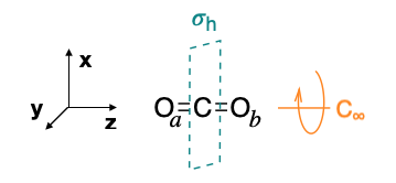
We can label the pendant atoms as \(\ce{O}_a\) and \(\ce{O}_b\), as in Figure \(\PageIndex{1}\).
Step 5.2: Create an expanded character table with one pendant atom's projected position for each operation
The \(D_{2h}\) character table needs no expansion because each operation is in its own class. We will arbitrarily choose to determine the new position of \(\ce{O}_a\) after each operation.
\[\begin{array}{|c|cccccccc|} \hline \bf{D_{2h}} & E & C_2(z) & C_2(y) &C_2(x) & i &\sigma(xy) & \sigma(xz) & \sigma(yz)\\ \hline \bf{\text{Projection of }\ce{O}_a} & \ce{O}_a & \ce{O}_a & \ce{O}_b & \ce{O}_b & \ce{O}_b & \ce{O}_b & \ce{O}_a & \ce{O}_a \\ \hline \end{array} \nonumber \]
Step 5.3: Find the contribution of each pendant atom to each SALC
Create a linear combination of the projections for each or the SALCs. The irreducible representations were found in step 4 in Section 5.4.2. Eight irreducible representations were found to be: \(2A_{g} + 2B_{1u} + B_{2g} + B_{3u} + B_{3g} + B_{2u}\). For each of the irreducible representations, multiply the projection by the respective character of the operation.
\[\text{Contribution of each atom to the SALC } = \sum(\text{Projection of }H_a \times \chi) \nonumber \]
The linear combination for all irreducible representations of \(D_{2h}\) are shown below.
\[\text{Table }\ref{expanded2} \text{: The symmetry adapted linear combination (SALC) for each irreducible representations of \(C_3v\) are shown.} \nonumber \]\[\begin{array}{|c|cccccccc|l|} \hline \bf{D_{2h}} & E & C_2(z) & C_2(y) &C_2(x) & i &\sigma(xy) & \sigma(xz) & \sigma(yz) & \text{Linear Combination} \\
\hline \bf{\text{Projection of }\ce{O}_a} &\bf \ce{O}_a &\bf \ce{O}_a &\bf \ce{O}_b &\bf \ce{O}_b &\bf \ce{O}_b &\bf \ce{O}_b &\bf \ce{O}_a &\bf \ce{O}_a \\
A_{g} & 1 & 1 & 1 & 1 & 1 & 1 & 1 & 1 & = \bf 4\ce{O}_a + 4\ce{O}_b \\
B_{1u} & 1 & 1 & -1 & -1 & -1 & -1 & 1 & 1 & = \bf 4\ce{O}_a - 4\ce{O}_b \\
B_{2g} & 1 & -1 & 1 & -1 & 1 & -1 & 1 & -1 & = \bf 0 \\
B_{3u} & 1 & -1 & -1 & 1 & -1 & 1 & 1 & -1 & = \bf 0\\
B_{3g} & 1 & -1 & -1 & 1 & 1 & -1 & -1 & 1 & = \bf 0\\
B_{2u} & 1 & -1 & 1 & -1 & -1 & 1 & -1 & 1 & = \bf 0\\
\hline \end{array} \label{expanded2} \]
Notice that there are only two irreducible representations that produce SALCs, the \(A_g\) and the \(B_{1u}\). Since we found two of each (\(2A_{g} + 2B_{1u}\)) when we found the irreducible representations, we know that there will be two SALCs of \(A_g\) symmetry and two of \(B_{1u}\) symmetry; that is four total SALCs from the pendant oxygens. This is the same as what we found in Section 5.4.2 using a different method.
Step 5.4: Sketch the SALCs
The SALCs with \(A_g\) symmetry: Quantitatively, we can apply the normalizing factor, N, for these SALCs. Each atom contributes equally to the SALCs, thus the normalizing factor for the \(A_g\) SALC is \(N=\left(\frac{1}{\sqrt{1^2 + 1^2}}\right) = \frac{1}{\sqrt{2}}\). This tells us that each oxygen contributes \(\frac{1}{\sqrt{2}}\) to each of the normalized \(A_g\) group orbitals: \[ A_g \text{ group orbital } = \frac{1}{\sqrt{2}}\left[\psi_{O_{a}}+\psi_{O_{b}}\right] \nonumber \]
The linear combination \(4\ce{O}_a + 4\ce{O}_b\) indicates that wavefunctions from each oxygen atom contribute equally to each of the two SALCs, with the same sign of the wavefunction for each. Because we know that \(A_g\) is totally symmetric (all 1's in the characters), we can assume that the SALC's will look like a symmetric arrangement of oxygen orbitals. But which orbitals contribute? We could peek at the character table to get a hint. But we'll treat this problem systematically.
The SALCs with \(B_{1u}\) symmetry: The linear combination \(4\ce{O}_a - 4\ce{O}_b\) indicates that each oxygen atom contributes equally, but that they have opposite wavefunctions. Application of the normalizing factor would give us: \[ B_{1u} \text{ group orbital } = \frac{1}{\sqrt{2}}\left[\psi_{O_{a}}+\psi_{O_{b}}\right] \nonumber \] But how do we know what the SALCs look like? Again, the character table can give us some hints, but we'll use a systematic process, below.
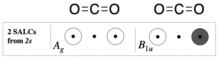
What do the SALCs look like? One way to systematically derive the SALC shapes is to perform the projection (Step 5.3) on specific groups of orbitals on the oxygen atom. For example, if we replicate Table \ref{expanded2} using just the group of oxygen 2s orbitals and the \(A_g\) and \(B_{1u}\) representations, we get the following:
\[\begin{array}{|c|cccccccc|l|} \hline \bf{D_{2h}} & E & C_2(z) & C_2(y) &C_2(x) & i &\sigma(xy) & \sigma(xz) & \sigma(yz) & \text{Linear Combination} \\
\hline \bf{\text{Projection of 2s orbital of }\ce{O}_a} &\bf \ce{O}1s_a &\bf \ce{O}1s_a &\bf \ce{O}1s_b &\bf \ce{O}1s_b &\bf \ce{O}1s_b &\bf \ce{O}1s_b &\bf \ce{O}1s_a &\bf \ce{O}1s_a \\
A_{g} & 1 & 1 & 1 & 1 & 1 & 1 & 1 & 1 & = \bf 4\ce{O}1s_a + 4\ce{O}1s_b \\
B_{1u} & 1 & 1 & -1 & -1 & -1 & -1 & 1 & 1 & = \bf 4\ce{O}1s_a - 4\ce{O}1s_b \\
\hline \end{array} \label{expanded3} \]
This tells us that one of the \(A_g\) SALCs looks like two oxygen 1s orbitals with equal signs and contributions. It also tells us that one of the \(B_{1u}\) SALCs looks like two \(s\) orbitals with opposite signs and equal magnitudes. These two SALCs are shown in Figure \(\PageIndex{2}\).
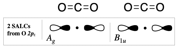
If we do the same for the \(2p_z\) orbitals, we need to pay attention to the orientation of the \(p\) orbital lobes. If the orbital is moved into the opposite orientation, it would get a negative sign in the projection (see below).
\[\begin{array}{|c|cccccccc|l|} \hline \bf{D_{2h}} & E & C_2(z) & C_2(y) &C_2(x) & i &\sigma(xy) & \sigma(xz) & \sigma(yz) & \text{Linear Combination} \\
\hline \bf{\text{Projection of 2px orbital of }\ce{O}_a} &\bf +\ce{O}2pz_a &\bf +\ce{O}2pz_a &\bf -\ce{O}2pz_b &\bf +\ce{O}2pz_b &\bf -\ce{O}2pz_b &\bf -\ce{O}2pz_b &\bf +\ce{O}2pz_a &\bf +\ce{O}2pz_a \\
A_{g} & 1 & 1 & 1 & 1 & 1 & 1 & 1 & 1 & = \bf 4\ce{O}2pz_a - 4\ce{O}2pz_b \\
B_{1u} & 1 & 1 & -1 & -1 & -1 & -1 & 1 & 1 & = \bf 4\ce{O}2pz_a + 4\ce{O}2pz_b \\
\hline \end{array} \label{expanded4} \]
This tells us that one of the \(A_g\) SALCs is derived from two \(2p_z\) orbitals of opposite sign but equal magnitude. In other words, the two \(p\) orbitals are pointing in opposite directions, but the lobes that are facing one another are of the same sign (see Figure \(\PageIndex{3}\), left). This also tells us that one of the \(B_{1u}\) orbitals is derived from two \(p_z\) orbitals of equal magnitude and equal sign (pointing in the same directions, with lobes facing one another of opposite sign!) (see Figure \(\PageIndex{3}\), right).
Now we have reached the same SALCs that we found previously in Section 5.4.2, but by an alternate method.