
5.2: The First Brillouin Zone
- Page ID
- 474776

\( \newcommand{\vecs}[1]{\overset { \scriptstyle \rightharpoonup} {\mathbf{#1}} } \)
\( \newcommand{\vecd}[1]{\overset{-\!-\!\rightharpoonup}{\vphantom{a}\smash {#1}}} \)
\( \newcommand{\id}{\mathrm{id}}\) \( \newcommand{\Span}{\mathrm{span}}\)
( \newcommand{\kernel}{\mathrm{null}\,}\) \( \newcommand{\range}{\mathrm{range}\,}\)
\( \newcommand{\RealPart}{\mathrm{Re}}\) \( \newcommand{\ImaginaryPart}{\mathrm{Im}}\)
\( \newcommand{\Argument}{\mathrm{Arg}}\) \( \newcommand{\norm}[1]{\| #1 \|}\)
\( \newcommand{\inner}[2]{\langle #1, #2 \rangle}\)
\( \newcommand{\Span}{\mathrm{span}}\)
\( \newcommand{\id}{\mathrm{id}}\)
\( \newcommand{\Span}{\mathrm{span}}\)
\( \newcommand{\kernel}{\mathrm{null}\,}\)
\( \newcommand{\range}{\mathrm{range}\,}\)
\( \newcommand{\RealPart}{\mathrm{Re}}\)
\( \newcommand{\ImaginaryPart}{\mathrm{Im}}\)
\( \newcommand{\Argument}{\mathrm{Arg}}\)
\( \newcommand{\norm}[1]{\| #1 \|}\)
\( \newcommand{\inner}[2]{\langle #1, #2 \rangle}\)
\( \newcommand{\Span}{\mathrm{span}}\) \( \newcommand{\AA}{\unicode[.8,0]{x212B}}\)
\( \newcommand{\vectorA}[1]{\vec{#1}} % arrow\)
\( \newcommand{\vectorAt}[1]{\vec{\text{#1}}} % arrow\)
\( \newcommand{\vectorB}[1]{\overset { \scriptstyle \rightharpoonup} {\mathbf{#1}} } \)
\( \newcommand{\vectorC}[1]{\textbf{#1}} \)
\( \newcommand{\vectorD}[1]{\overrightarrow{#1}} \)
\( \newcommand{\vectorDt}[1]{\overrightarrow{\text{#1}}} \)
\( \newcommand{\vectE}[1]{\overset{-\!-\!\rightharpoonup}{\vphantom{a}\smash{\mathbf {#1}}}} \)
\( \newcommand{\vecs}[1]{\overset { \scriptstyle \rightharpoonup} {\mathbf{#1}} } \)
\( \newcommand{\vecd}[1]{\overset{-\!-\!\rightharpoonup}{\vphantom{a}\smash {#1}}} \)
\(\newcommand{\avec}{\mathbf a}\) \(\newcommand{\bvec}{\mathbf b}\) \(\newcommand{\cvec}{\mathbf c}\) \(\newcommand{\dvec}{\mathbf d}\) \(\newcommand{\dtil}{\widetilde{\mathbf d}}\) \(\newcommand{\evec}{\mathbf e}\) \(\newcommand{\fvec}{\mathbf f}\) \(\newcommand{\nvec}{\mathbf n}\) \(\newcommand{\pvec}{\mathbf p}\) \(\newcommand{\qvec}{\mathbf q}\) \(\newcommand{\svec}{\mathbf s}\) \(\newcommand{\tvec}{\mathbf t}\) \(\newcommand{\uvec}{\mathbf u}\) \(\newcommand{\vvec}{\mathbf v}\) \(\newcommand{\wvec}{\mathbf w}\) \(\newcommand{\xvec}{\mathbf x}\) \(\newcommand{\yvec}{\mathbf y}\) \(\newcommand{\zvec}{\mathbf z}\) \(\newcommand{\rvec}{\mathbf r}\) \(\newcommand{\mvec}{\mathbf m}\) \(\newcommand{\zerovec}{\mathbf 0}\) \(\newcommand{\onevec}{\mathbf 1}\) \(\newcommand{\real}{\mathbb R}\) \(\newcommand{\twovec}[2]{\left[\begin{array}{r}#1 \\ #2 \end{array}\right]}\) \(\newcommand{\ctwovec}[2]{\left[\begin{array}{c}#1 \\ #2 \end{array}\right]}\) \(\newcommand{\threevec}[3]{\left[\begin{array}{r}#1 \\ #2 \\ #3 \end{array}\right]}\) \(\newcommand{\cthreevec}[3]{\left[\begin{array}{c}#1 \\ #2 \\ #3 \end{array}\right]}\) \(\newcommand{\fourvec}[4]{\left[\begin{array}{r}#1 \\ #2 \\ #3 \\ #4 \end{array}\right]}\) \(\newcommand{\cfourvec}[4]{\left[\begin{array}{c}#1 \\ #2 \\ #3 \\ #4 \end{array}\right]}\) \(\newcommand{\fivevec}[5]{\left[\begin{array}{r}#1 \\ #2 \\ #3 \\ #4 \\ #5 \\ \end{array}\right]}\) \(\newcommand{\cfivevec}[5]{\left[\begin{array}{c}#1 \\ #2 \\ #3 \\ #4 \\ #5 \\ \end{array}\right]}\) \(\newcommand{\mattwo}[4]{\left[\begin{array}{rr}#1 \amp #2 \\ #3 \amp #4 \\ \end{array}\right]}\) \(\newcommand{\laspan}[1]{\text{Span}\{#1\}}\) \(\newcommand{\bcal}{\cal B}\) \(\newcommand{\ccal}{\cal C}\) \(\newcommand{\scal}{\cal S}\) \(\newcommand{\wcal}{\cal W}\) \(\newcommand{\ecal}{\cal E}\) \(\newcommand{\coords}[2]{\left\{#1\right\}_{#2}}\) \(\newcommand{\gray}[1]{\color{gray}{#1}}\) \(\newcommand{\lgray}[1]{\color{lightgray}{#1}}\) \(\newcommand{\rank}{\operatorname{rank}}\) \(\newcommand{\row}{\text{Row}}\) \(\newcommand{\col}{\text{Col}}\) \(\renewcommand{\row}{\text{Row}}\) \(\newcommand{\nul}{\text{Nul}}\) \(\newcommand{\var}{\text{Var}}\) \(\newcommand{\corr}{\text{corr}}\) \(\newcommand{\len}[1]{\left|#1\right|}\) \(\newcommand{\bbar}{\overline{\bvec}}\) \(\newcommand{\bhat}{\widehat{\bvec}}\) \(\newcommand{\bperp}{\bvec^\perp}\) \(\newcommand{\xhat}{\widehat{\xvec}}\) \(\newcommand{\vhat}{\widehat{\vvec}}\) \(\newcommand{\uhat}{\widehat{\uvec}}\) \(\newcommand{\what}{\widehat{\wvec}}\) \(\newcommand{\Sighat}{\widehat{\Sigma}}\) \(\newcommand{\lt}{<}\) \(\newcommand{\gt}{>}\) \(\newcommand{\amp}{&}\) \(\definecolor{fillinmathshade}{gray}{0.9}\)There are two important corollaries of Bloch’s theorem that will be important for solving the Schrödinger equation for electronic and vibrational states in crystals:
- If \(\boldsymbol{K}\) is a reciprocal lattice vector, then the Bloch functions \(\psi_{n\boldsymbol{k}}\left( \boldsymbol{r} \right)\) and \(\psi_{n(\boldsymbol{k} + \boldsymbol{K})}\left( \boldsymbol{r} \right)\) are basis functions for the same IR \(\Gamma^{(\boldsymbol{k})}\). That is, these functions are transformed identically by the same lattice translation. Consider each of these two Bloch functions evaluated at \(\boldsymbol{r} + \boldsymbol{T}\):
\(\psi_{n\boldsymbol{k}}\left( \boldsymbol{r} + \boldsymbol{T} \right) = e^{i\boldsymbol{k} \cdot \boldsymbol{T}}\psi_{n\boldsymbol{k}}(\boldsymbol{r})\) and
\(\psi_{n(\boldsymbol{k} + \boldsymbol{K})}\left( \boldsymbol{r} + \boldsymbol{T} \right) = e^{i(\boldsymbol{k} + \boldsymbol{K}) \cdot \boldsymbol{T}}\psi_{n(\boldsymbol{k} + \boldsymbol{K})}\left( \boldsymbol{r} \right) = e^{i\boldsymbol{k} \cdot \boldsymbol{T}}e^{i\boldsymbol{K} \cdot \boldsymbol{T}}\psi_{n(\boldsymbol{k} + \boldsymbol{K})}\left( \boldsymbol{r} \right) = e^{i\boldsymbol{k} \cdot \boldsymbol{T}}\psi_{n(\boldsymbol{k} + \boldsymbol{K})}\left( \boldsymbol{r} \right)\)
Therefore, \(\psi_{n\boldsymbol{k}}\left( \boldsymbol{r} \right)\) and \(\psi_{n(\boldsymbol{k} + \boldsymbol{K})}\left( \boldsymbol{r} \right)\) show the same change in phase factor when \(\boldsymbol{r}\) is shifted to \(\boldsymbol{r} + \boldsymbol{T}\). Nevertheless, these two functions are distinct basis functions for the same IR \(\Gamma^{(\boldsymbol{k})}\).
- The Bloch function \(\psi_{n( - \boldsymbol{k})}\left( \boldsymbol{r} \right)\) and the complex conjugate function \(\psi_{n\boldsymbol{k}}^{*}\left( \boldsymbol{r} \right)\) are basis functions for the same IR \(\Gamma^{( - \boldsymbol{k})}\), as seen as follows:
\(\psi_{n( - \boldsymbol{k})}\left( \boldsymbol{r} + \boldsymbol{T} \right) = e^{i( - \boldsymbol{k}) \cdot \boldsymbol{T}}\psi_{n( - \boldsymbol{k})}\left( \boldsymbol{r} \right) = e^{- i\boldsymbol{k} \cdot \boldsymbol{T}}\psi_{n( - \boldsymbol{k})}\left( \boldsymbol{r} \right)\), and
\(\psi_{n\boldsymbol{k}}^{*}\left( \boldsymbol{r} + \boldsymbol{T} \right) = \left\lbrack e^{i\boldsymbol{k} \cdot \boldsymbol{T}}\psi_{n\boldsymbol{k}}\left( \boldsymbol{r} \right) \right\rbrack^{*} = e^{- i\boldsymbol{k} \cdot \boldsymbol{T}}\psi_{n\boldsymbol{k}}^{*}\left( \boldsymbol{r} \right)\).
Moreover, the IR \(\Gamma^{( - \boldsymbol{k})}\) is complex conjugate to \(\Gamma^{(\boldsymbol{k})}\):
\[\Gamma^{\left( \boldsymbol{k} \right)}\left( 1 \middle| \boldsymbol{T} \right) = e^{- i\boldsymbol{k} \cdot \boldsymbol{T}}\) and \(\Gamma^{\left( - \boldsymbol{k} \right)}\left( 1 \middle| \boldsymbol{T} \right) = e^{- ( - \boldsymbol{k}) \cdot \boldsymbol{T}} = e^{i\boldsymbol{k} \cdot \boldsymbol{T}} = \left\lbrack \Gamma^{\left( \boldsymbol{k} \right)}\left( 1 \middle| \boldsymbol{T} \right) \right\rbrack^{*}. \nonumber \]
It is not necessary that \(\psi_{n( - \boldsymbol{k})}\left( \boldsymbol{r} \right) = \psi_{n\boldsymbol{k}}^{*}\left( \boldsymbol{r} \right)\). Nevertheless, since \(\psi_{n( - \boldsymbol{k})}\left( \boldsymbol{r} \right)\) and \(\psi_{n\boldsymbol{k}}^{*}\left( \boldsymbol{r} \right)\) are basis functions for the same IR \(\Gamma^{( - \boldsymbol{k})}\), \(\psi_{n( - \boldsymbol{k})}\left( \boldsymbol{r} \right)\) and \(\psi_{n\boldsymbol{k}}\left( \boldsymbol{r} \right)\) are degenerate eigenfunctions of the Hermitian Hamiltonian operator, so that \(E_{n}\left( - \boldsymbol{k} \right) = E_{n}\left( \boldsymbol{k} \right)\).
Bloch functions for the 1-d lattice
Before discussing some important ramifications of these corollaries, let’s examine Bloch functions for the 1-d lattice using the periodic boundary condition \(\boldsymbol{T}_{4} = \left( 1 \middle| 4\boldsymbol{a} \right) \equiv \left( 1 \middle| \mathbf{0} \right) = \boldsymbol{T}_{0}\). According to Part IV, \(\mathbf{\Gamma}^{(\mu)} = e^{- ik_{\mu}ma}\) for wavevectors \(k_{\mu} = \frac{\mu}{4}\left( \frac{2\pi}{a} \right);\ \mu = 0,\ 1,\ 2,\ 3\):
@ >p(- 14) * >p(- 14) * >p(- 14) * >p(- 14) * >p(- 14) * >p(- 14) * >p(- 14) * >p(- 14) * @
()
\[\mathcal{L} \nonumber \]
&
\[\boldsymbol{T}_{0} \nonumber \]
&
\[\boldsymbol{T}_{1} \nonumber \]
&
\[\boldsymbol{T}_{2} \nonumber \]
&
\[\boldsymbol{T}_{3} \nonumber \]
&
() ()
\[\mathcal{L} \nonumber \]
&
\[\boldsymbol{T}_{0} \nonumber \]
&
\[\boldsymbol{T}_{1} \nonumber \]
&
\[\boldsymbol{T}_{2} \nonumber \]
&
\[\boldsymbol{T}_{3} \nonumber \]
&
() \(k_{\mu}\) (Wavevector) & Real: \(\cos{k_{\mu}x}\) & Imaginary: \(\sin{k_{\mu}x}\) & & & & &
& & & & & \(k_{0} = \frac{0}{4}\left( \frac{2\pi}{a} \right) = 0\) & 
Figure 5.1 & 
Figure 5.2
& & & & & \(k_{4} \equiv k_{0} + K_{1} = \frac{2\pi}{a}\) & 
Figure 5.3 & 
Figure 5.4
\(\mathbf{\Gamma}^{(1)}\) & +1 & –i & –1 & +i & \(k_{1} = \frac{1}{4}\left( \frac{2\pi}{a} \right) = \frac{\pi}{2a}\) & 
Figure 5.5 & 
Figure 5.6
\(\mathbf{\Gamma}^{\mathbf{(}\mathbf{2}\mathbf{)}}\) & +1 & –1 & +1 & –1 & \(k_{2} = \frac{2}{4}\left( \frac{2\pi}{a} \right) = \frac{\pi}{a}\) & 
Figure 5.7 & 
Figure 5.8
& & & & & \(k_{3} = \frac{3}{4}\left( \frac{2\pi}{a} \right) = \frac{3\pi}{2a}\) & 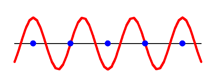
Figure 5.9 & 
Figure 5.10
& & & & & \(k_{- 1} \equiv k_{3} - K_{1} = \frac{- \pi}{2a}\) & 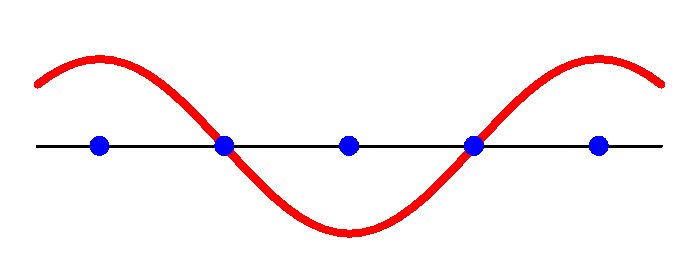
Figure 5.11 & 
Figure 5.12
& & & & & &  &
& 
()
Some outcomes of this table include:
- The Bloch functions \(\psi_{k_{0}}(x)\) and \(\psi_{k_{0} + K_{1}}(x)\) where \(K_{1} = \frac{2\pi}{a}\) are distinct basis functions for the IR \(\mathbf{\Gamma}^{(0)}\). Since \(k_{0} + K_{1} = \frac{2\pi}{a}\), we can write \(k_{0} + K_{1} \equiv k_{4}\).
- The Bloch functions \(\psi_{k_{3}}(x)\) and \(\psi_{k_{3} - K_{1}}(x)\) where \(K_{1} = \frac{2\pi}{a}\) are distinct basis functions for the IR \(\mathbf{\Gamma}^{(3)}\). Since \(k_{3} - K_{1} = \frac{- \pi}{2a}\), we can write \(k_{3} - K_{1} \equiv k_{- 1}\).
- \(\mathbf{\Gamma}^{(1)}\) and \(\mathbf{\Gamma}^{(3)}\) are complex conjugate IRs; the basis functions, \(\psi_{k_{3}}(x)\) and \(\psi_{k_{- 1}}(x)\), are complex conjugates of each other.
Bloch’s theorem and its corollaries indicate that the wavevectors that label the IRs of the group of lattice translations fall within any single unit cell of the reciprocal lattice. This region, which is chosen to be the Wigner-Seitz cell of the reciprocal lattice point \(\mathbf{K}_{000} = \mathbf{0}\), is called the first Brillouin zone. These regions are illustrated below for various 1-d, 2-d, and 3-d reciprocal lattices.
1-d Lattice (Rotational Symmetry \(\bf{\overline{1}}\)):

The first Brillouin zone contains wavevectors \(\frac{- \pi}{a} < k_{\mu} \leq \frac{\pi}{a}\). The two boundary points are equivalent because they differ by the reciprocal lattice vector \(K_{1} = \frac{2\pi}{a}\). When solving the Schrödinger equation for problems involving 1-d lattices, the second corollary of Bloch’s theorem reduces this region to \(0 \leq k_{\mu} \leq \frac{\pi}{a}\), called the irreducible wedge. Certain wavevectors get special labels, e.g., \(\Gamma = 0\) and \(X = \frac{\pi}{a}\).
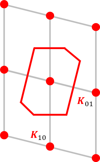
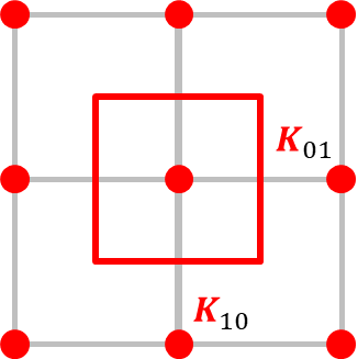
2-d Lattices:
@ >p(- 8) * >p(- 8) * >p(- 8) * >p(- 8) * >p(- 8) * @
()

Oblique (2)
\(a_{1}^{\ast}\)a1∗ > \(a_{2}^{\ast}\)a2∗
&
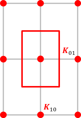
Rectangular (2mm)
\(a_{1}^{\ast} > a_{2}^{\ast}\)a1∗>a2∗
&

Centered Rectangular (2mm)
&

Tetragonal (4mm)
&
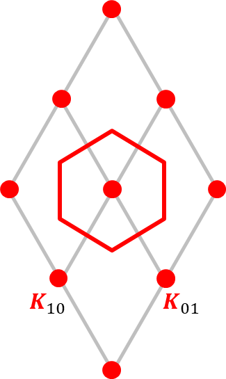
Hexagonal (6mm) and Trigonal
() ()
Oblique (2)
\(a_{1}^{\ast}\)a1∗ > \(a_{2}^{\ast}\)a2∗
&

Rectangular (2mm)
\(a_{1}^{\ast} > a_{2}^{\ast}\)a1∗>a2∗
&

Centered Rectangular (2mm)
&
Tetragonal (4mm)
&

Hexagonal (6mm) and Trigonal
() ()
The first Brillouin zones have the full rotational symmetries of their corresponding lattices. Their irreducible wedges, which will be discussed in more detail in the next section, take into account the second corollary as well as rotational symmetry.
Selected 3-d Lattices:

Simple Cubic (\(m\bar{3}m\)m3m)

Simple Hexagonal
(6/mmm; \(a_{3}^{\ast}\)a3∗ < \(a_{1}^{\ast}\)a1∗ )
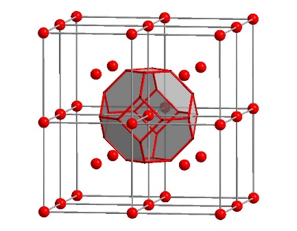
Body-Centered Cubic (\(m\bar{3}m\)m3m)
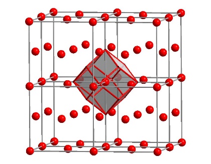
Figure 5.22:
Face-Centered Cubic (\(m\bar{3}m\)m3m)