21.3: Atomic Spectra and the Bohr Theory
- Page ID
- 49637
\( \newcommand{\vecs}[1]{\overset { \scriptstyle \rightharpoonup} {\mathbf{#1}} } \)
\( \newcommand{\vecd}[1]{\overset{-\!-\!\rightharpoonup}{\vphantom{a}\smash {#1}}} \)
\( \newcommand{\id}{\mathrm{id}}\) \( \newcommand{\Span}{\mathrm{span}}\)
( \newcommand{\kernel}{\mathrm{null}\,}\) \( \newcommand{\range}{\mathrm{range}\,}\)
\( \newcommand{\RealPart}{\mathrm{Re}}\) \( \newcommand{\ImaginaryPart}{\mathrm{Im}}\)
\( \newcommand{\Argument}{\mathrm{Arg}}\) \( \newcommand{\norm}[1]{\| #1 \|}\)
\( \newcommand{\inner}[2]{\langle #1, #2 \rangle}\)
\( \newcommand{\Span}{\mathrm{span}}\)
\( \newcommand{\id}{\mathrm{id}}\)
\( \newcommand{\Span}{\mathrm{span}}\)
\( \newcommand{\kernel}{\mathrm{null}\,}\)
\( \newcommand{\range}{\mathrm{range}\,}\)
\( \newcommand{\RealPart}{\mathrm{Re}}\)
\( \newcommand{\ImaginaryPart}{\mathrm{Im}}\)
\( \newcommand{\Argument}{\mathrm{Arg}}\)
\( \newcommand{\norm}[1]{\| #1 \|}\)
\( \newcommand{\inner}[2]{\langle #1, #2 \rangle}\)
\( \newcommand{\Span}{\mathrm{span}}\) \( \newcommand{\AA}{\unicode[.8,0]{x212B}}\)
\( \newcommand{\vectorA}[1]{\vec{#1}} % arrow\)
\( \newcommand{\vectorAt}[1]{\vec{\text{#1}}} % arrow\)
\( \newcommand{\vectorB}[1]{\overset { \scriptstyle \rightharpoonup} {\mathbf{#1}} } \)
\( \newcommand{\vectorC}[1]{\textbf{#1}} \)
\( \newcommand{\vectorD}[1]{\overrightarrow{#1}} \)
\( \newcommand{\vectorDt}[1]{\overrightarrow{\text{#1}}} \)
\( \newcommand{\vectE}[1]{\overset{-\!-\!\rightharpoonup}{\vphantom{a}\smash{\mathbf {#1}}}} \)
\( \newcommand{\vecs}[1]{\overset { \scriptstyle \rightharpoonup} {\mathbf{#1}} } \)
\( \newcommand{\vecd}[1]{\overset{-\!-\!\rightharpoonup}{\vphantom{a}\smash {#1}}} \)
\(\newcommand{\avec}{\mathbf a}\) \(\newcommand{\bvec}{\mathbf b}\) \(\newcommand{\cvec}{\mathbf c}\) \(\newcommand{\dvec}{\mathbf d}\) \(\newcommand{\dtil}{\widetilde{\mathbf d}}\) \(\newcommand{\evec}{\mathbf e}\) \(\newcommand{\fvec}{\mathbf f}\) \(\newcommand{\nvec}{\mathbf n}\) \(\newcommand{\pvec}{\mathbf p}\) \(\newcommand{\qvec}{\mathbf q}\) \(\newcommand{\svec}{\mathbf s}\) \(\newcommand{\tvec}{\mathbf t}\) \(\newcommand{\uvec}{\mathbf u}\) \(\newcommand{\vvec}{\mathbf v}\) \(\newcommand{\wvec}{\mathbf w}\) \(\newcommand{\xvec}{\mathbf x}\) \(\newcommand{\yvec}{\mathbf y}\) \(\newcommand{\zvec}{\mathbf z}\) \(\newcommand{\rvec}{\mathbf r}\) \(\newcommand{\mvec}{\mathbf m}\) \(\newcommand{\zerovec}{\mathbf 0}\) \(\newcommand{\onevec}{\mathbf 1}\) \(\newcommand{\real}{\mathbb R}\) \(\newcommand{\twovec}[2]{\left[\begin{array}{r}#1 \\ #2 \end{array}\right]}\) \(\newcommand{\ctwovec}[2]{\left[\begin{array}{c}#1 \\ #2 \end{array}\right]}\) \(\newcommand{\threevec}[3]{\left[\begin{array}{r}#1 \\ #2 \\ #3 \end{array}\right]}\) \(\newcommand{\cthreevec}[3]{\left[\begin{array}{c}#1 \\ #2 \\ #3 \end{array}\right]}\) \(\newcommand{\fourvec}[4]{\left[\begin{array}{r}#1 \\ #2 \\ #3 \\ #4 \end{array}\right]}\) \(\newcommand{\cfourvec}[4]{\left[\begin{array}{c}#1 \\ #2 \\ #3 \\ #4 \end{array}\right]}\) \(\newcommand{\fivevec}[5]{\left[\begin{array}{r}#1 \\ #2 \\ #3 \\ #4 \\ #5 \\ \end{array}\right]}\) \(\newcommand{\cfivevec}[5]{\left[\begin{array}{c}#1 \\ #2 \\ #3 \\ #4 \\ #5 \\ \end{array}\right]}\) \(\newcommand{\mattwo}[4]{\left[\begin{array}{rr}#1 \amp #2 \\ #3 \amp #4 \\ \end{array}\right]}\) \(\newcommand{\laspan}[1]{\text{Span}\{#1\}}\) \(\newcommand{\bcal}{\cal B}\) \(\newcommand{\ccal}{\cal C}\) \(\newcommand{\scal}{\cal S}\) \(\newcommand{\wcal}{\cal W}\) \(\newcommand{\ecal}{\cal E}\) \(\newcommand{\coords}[2]{\left\{#1\right\}_{#2}}\) \(\newcommand{\gray}[1]{\color{gray}{#1}}\) \(\newcommand{\lgray}[1]{\color{lightgray}{#1}}\) \(\newcommand{\rank}{\operatorname{rank}}\) \(\newcommand{\row}{\text{Row}}\) \(\newcommand{\col}{\text{Col}}\) \(\renewcommand{\row}{\text{Row}}\) \(\newcommand{\nul}{\text{Nul}}\) \(\newcommand{\var}{\text{Var}}\) \(\newcommand{\corr}{\text{corr}}\) \(\newcommand{\len}[1]{\left|#1\right|}\) \(\newcommand{\bbar}{\overline{\bvec}}\) \(\newcommand{\bhat}{\widehat{\bvec}}\) \(\newcommand{\bperp}{\bvec^\perp}\) \(\newcommand{\xhat}{\widehat{\xvec}}\) \(\newcommand{\vhat}{\widehat{\vvec}}\) \(\newcommand{\uhat}{\widehat{\uvec}}\) \(\newcommand{\what}{\widehat{\wvec}}\) \(\newcommand{\Sighat}{\widehat{\Sigma}}\) \(\newcommand{\lt}{<}\) \(\newcommand{\gt}{>}\) \(\newcommand{\amp}{&}\) \(\definecolor{fillinmathshade}{gray}{0.9}\)When any element is heated to a sufficiently high temperature, all bonds between atoms are dissociated and the element turns into a monatomic gas. At these or still higher temperatures the single atoms begin to radiate visible and ultraviolet light. The actual pattern of light emitted varies from element to element and is called its emission spectrum. Such a spectrum is commonly obtained by passing an electric arc through a powdered sample of the solid element or by applying a voltage to a discharge tube containing a gas at low pressure. Neon signs are everyday examples of discharge tubes. Neon produces a bright red glow in the tube, and other gases produce different colors.

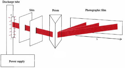
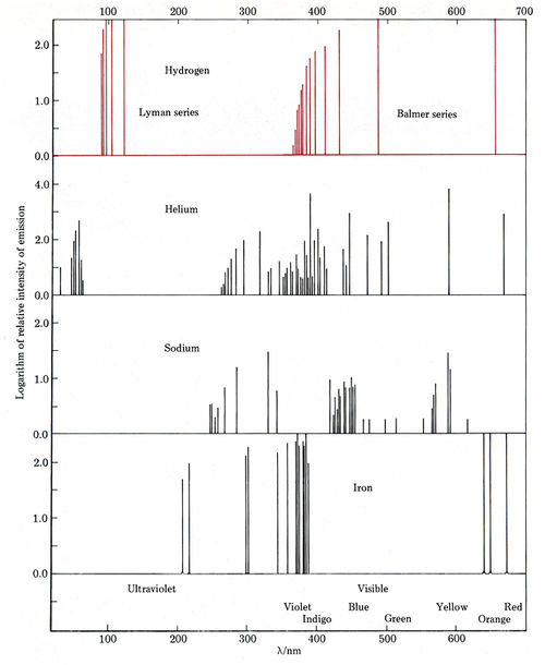
If the emission spectrum of an element is passed through a prism and allowed to strike a photographic film, the intensity of emission as a function of wavelength can be measured. The equipment for making such measurements is called a spectroscope and is shown schematically in Figure \(\PageIndex{1}\). Typical emission spectra obtained in this way are shown in Figure \(\PageIndex{2}\) where the intensity is plotted against wavelength. Note from this figure how the light emitted is confined to a few very specific wavelengths. At all other wavelengths there is no emission at all. Spectra of this kind are usually referred to as line spectra. The wavelengths of the lines in a line spectrum are unique to each element and are often used, especially in metallurgy, both to identify an element and to measure the amount present. These wavelengths can often be measured to an accuracy as great as one part in a billion (1 in 109). Because the spectrum of an element is readily reproducible and can be measured so accurately, it is often used to determine lengths. For example, the meter was once defined as the distance between two marks on a platinum bar kept at Sevrés in France, but now it is taken as 1 650 763.73 wavelengths of a particular line in the spectrum of 86Kr.
At first glance the wavelengths of the lines in an emission spectrum, like those shown in Figure \(\PageIndex{2}\), appear to have no pattern to them, but upon closer study regularities can be distinguished.

For example, you can see that lines in the hydrogen spectrum occur very close together in the region just above 365 nm and then are spaced farther and farther apart as λ increases. In 1885 a Swiss high-school mathematics teacher, J. J. Balmer (1825 to 1898), discovered a formula which accounted for this regularity:
-
- \[\lambda=364.6 \text{ nm}\frac{n^{2}}{n^{2}-4} ~~~~ n = 3, 4, 5, \cdots \label{1} \]
When the number n is any positive integer greater than 2, the formula predicts a line in the hydrogen spectrum. For n = 3, the Balmer formula gives λ = 656.3 nm; when n = 4, λ = 486.1 nm; and so on. All spectral lines predicted by the Balmer formula are said to belong to the Balmer series.
Other similar series of lines are found in the ultraviolet (Lyman series) and infrared (Paschen, Brackett, Pfund series) regions of the spectrum. In each case the wavelengths of the lines can be predicted by an equation similar in form to Balmer’s. These equations were combined by Rydberg into the general form
-
- \[\frac{1}{\lambda}=R_{\infty}\big(\frac{1}{n_{1}^{2}}-\frac{1}{n_{2}^{2}}\big) ~~~~~~ n_2 \text{>} n_1 \label{2} \]
where R∞, called the Rydberg constant , has the value 1.097 094 × 107 m–1. Thus a single equation containing only one constant and two-integer parameters is able to predict virtually all the lines in the spectrum of atomic hydrogen.


