16.5: Thermodynamic Probability W and Entropy
- Page ID
- 49564
\( \newcommand{\vecs}[1]{\overset { \scriptstyle \rightharpoonup} {\mathbf{#1}} } \)
\( \newcommand{\vecd}[1]{\overset{-\!-\!\rightharpoonup}{\vphantom{a}\smash {#1}}} \)
\( \newcommand{\id}{\mathrm{id}}\) \( \newcommand{\Span}{\mathrm{span}}\)
( \newcommand{\kernel}{\mathrm{null}\,}\) \( \newcommand{\range}{\mathrm{range}\,}\)
\( \newcommand{\RealPart}{\mathrm{Re}}\) \( \newcommand{\ImaginaryPart}{\mathrm{Im}}\)
\( \newcommand{\Argument}{\mathrm{Arg}}\) \( \newcommand{\norm}[1]{\| #1 \|}\)
\( \newcommand{\inner}[2]{\langle #1, #2 \rangle}\)
\( \newcommand{\Span}{\mathrm{span}}\)
\( \newcommand{\id}{\mathrm{id}}\)
\( \newcommand{\Span}{\mathrm{span}}\)
\( \newcommand{\kernel}{\mathrm{null}\,}\)
\( \newcommand{\range}{\mathrm{range}\,}\)
\( \newcommand{\RealPart}{\mathrm{Re}}\)
\( \newcommand{\ImaginaryPart}{\mathrm{Im}}\)
\( \newcommand{\Argument}{\mathrm{Arg}}\)
\( \newcommand{\norm}[1]{\| #1 \|}\)
\( \newcommand{\inner}[2]{\langle #1, #2 \rangle}\)
\( \newcommand{\Span}{\mathrm{span}}\) \( \newcommand{\AA}{\unicode[.8,0]{x212B}}\)
\( \newcommand{\vectorA}[1]{\vec{#1}} % arrow\)
\( \newcommand{\vectorAt}[1]{\vec{\text{#1}}} % arrow\)
\( \newcommand{\vectorB}[1]{\overset { \scriptstyle \rightharpoonup} {\mathbf{#1}} } \)
\( \newcommand{\vectorC}[1]{\textbf{#1}} \)
\( \newcommand{\vectorD}[1]{\overrightarrow{#1}} \)
\( \newcommand{\vectorDt}[1]{\overrightarrow{\text{#1}}} \)
\( \newcommand{\vectE}[1]{\overset{-\!-\!\rightharpoonup}{\vphantom{a}\smash{\mathbf {#1}}}} \)
\( \newcommand{\vecs}[1]{\overset { \scriptstyle \rightharpoonup} {\mathbf{#1}} } \)
\( \newcommand{\vecd}[1]{\overset{-\!-\!\rightharpoonup}{\vphantom{a}\smash {#1}}} \)
\(\newcommand{\avec}{\mathbf a}\) \(\newcommand{\bvec}{\mathbf b}\) \(\newcommand{\cvec}{\mathbf c}\) \(\newcommand{\dvec}{\mathbf d}\) \(\newcommand{\dtil}{\widetilde{\mathbf d}}\) \(\newcommand{\evec}{\mathbf e}\) \(\newcommand{\fvec}{\mathbf f}\) \(\newcommand{\nvec}{\mathbf n}\) \(\newcommand{\pvec}{\mathbf p}\) \(\newcommand{\qvec}{\mathbf q}\) \(\newcommand{\svec}{\mathbf s}\) \(\newcommand{\tvec}{\mathbf t}\) \(\newcommand{\uvec}{\mathbf u}\) \(\newcommand{\vvec}{\mathbf v}\) \(\newcommand{\wvec}{\mathbf w}\) \(\newcommand{\xvec}{\mathbf x}\) \(\newcommand{\yvec}{\mathbf y}\) \(\newcommand{\zvec}{\mathbf z}\) \(\newcommand{\rvec}{\mathbf r}\) \(\newcommand{\mvec}{\mathbf m}\) \(\newcommand{\zerovec}{\mathbf 0}\) \(\newcommand{\onevec}{\mathbf 1}\) \(\newcommand{\real}{\mathbb R}\) \(\newcommand{\twovec}[2]{\left[\begin{array}{r}#1 \\ #2 \end{array}\right]}\) \(\newcommand{\ctwovec}[2]{\left[\begin{array}{c}#1 \\ #2 \end{array}\right]}\) \(\newcommand{\threevec}[3]{\left[\begin{array}{r}#1 \\ #2 \\ #3 \end{array}\right]}\) \(\newcommand{\cthreevec}[3]{\left[\begin{array}{c}#1 \\ #2 \\ #3 \end{array}\right]}\) \(\newcommand{\fourvec}[4]{\left[\begin{array}{r}#1 \\ #2 \\ #3 \\ #4 \end{array}\right]}\) \(\newcommand{\cfourvec}[4]{\left[\begin{array}{c}#1 \\ #2 \\ #3 \\ #4 \end{array}\right]}\) \(\newcommand{\fivevec}[5]{\left[\begin{array}{r}#1 \\ #2 \\ #3 \\ #4 \\ #5 \\ \end{array}\right]}\) \(\newcommand{\cfivevec}[5]{\left[\begin{array}{c}#1 \\ #2 \\ #3 \\ #4 \\ #5 \\ \end{array}\right]}\) \(\newcommand{\mattwo}[4]{\left[\begin{array}{rr}#1 \amp #2 \\ #3 \amp #4 \\ \end{array}\right]}\) \(\newcommand{\laspan}[1]{\text{Span}\{#1\}}\) \(\newcommand{\bcal}{\cal B}\) \(\newcommand{\ccal}{\cal C}\) \(\newcommand{\scal}{\cal S}\) \(\newcommand{\wcal}{\cal W}\) \(\newcommand{\ecal}{\cal E}\) \(\newcommand{\coords}[2]{\left\{#1\right\}_{#2}}\) \(\newcommand{\gray}[1]{\color{gray}{#1}}\) \(\newcommand{\lgray}[1]{\color{lightgray}{#1}}\) \(\newcommand{\rank}{\operatorname{rank}}\) \(\newcommand{\row}{\text{Row}}\) \(\newcommand{\col}{\text{Col}}\) \(\renewcommand{\row}{\text{Row}}\) \(\newcommand{\nul}{\text{Nul}}\) \(\newcommand{\var}{\text{Var}}\) \(\newcommand{\corr}{\text{corr}}\) \(\newcommand{\len}[1]{\left|#1\right|}\) \(\newcommand{\bbar}{\overline{\bvec}}\) \(\newcommand{\bhat}{\widehat{\bvec}}\) \(\newcommand{\bperp}{\bvec^\perp}\) \(\newcommand{\xhat}{\widehat{\xvec}}\) \(\newcommand{\vhat}{\widehat{\vvec}}\) \(\newcommand{\uhat}{\widehat{\uvec}}\) \(\newcommand{\what}{\widehat{\wvec}}\) \(\newcommand{\Sighat}{\widehat{\Sigma}}\) \(\newcommand{\lt}{<}\) \(\newcommand{\gt}{>}\) \(\newcommand{\amp}{&}\) \(\definecolor{fillinmathshade}{gray}{0.9}\)The section on atoms, molecules and probability has shown that if we want to predict whether a chemical change is spontaneous or not, we must find some general way of determining whether the final state is more probable than the initial. This can be done using a number W, called the thermodynamic probability. W is defined as the number of alternative microscopic arrangements which correspond to the same macroscopic state. The significance of this definition becomes more apparent once we have considered a few examples.
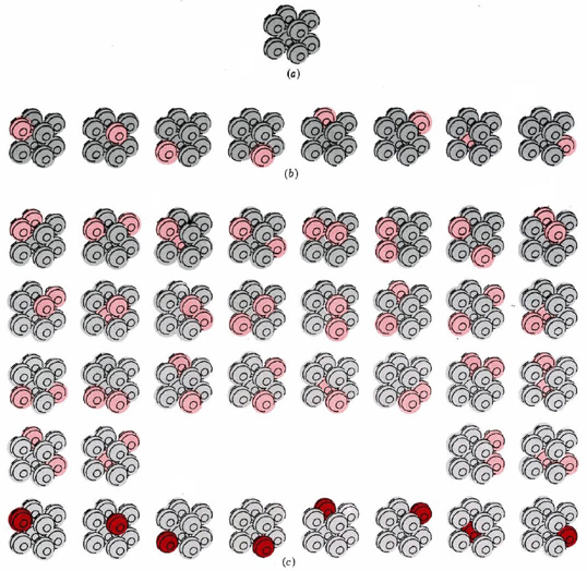
Figure \(\PageIndex{1}\) a illustrates a crystal consisting of only eight atoms at the absolute zero of temperature. Suppose that the temperature is raised slightly by supplying just enough energy to set one of the atoms in the crystal vibrating. There are eight possible ways of doing this, since we could supply the energy to any one of the eight atoms. All eight possibilities are shown in Figure \(\PageIndex{1}\) b.

Since all eight possibilities correspond to the crystal having the same temperature, we say that W = 8 for the crystal at this temperature. Also, we must realize that the crystal will not stay perpetually in any of these eight arrangements. Energy will constantly be transferred from one atom to the other, so that all the eight arrangements are equally probable.
Let us now supply a second quantity of energy exactly equal to the first, so that there is just enough to start two molecules vibrating. There are 36 different ways in which this energy can be assigned to the eight atoms (Figure \(\PageIndex{1}\) c). We say that W = 36 for the crystal at this second temperature. Because energy continually exchanges from one atom to another, there is an equal probability of finding the crystal in any of the 36 possible arrangements.
A third example of W is our eight-atom crystal at the absolute zero of temperature. Since there is no energy to be exchanged from atom to atom, only one arrangement is possible, and W = 1. This is true not only for this hypothetical crystal, but also presumably for a real crystal containing a large number of atoms, perfectly arranged, at absolute zero.

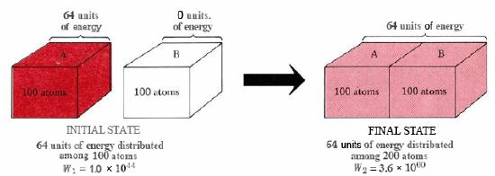
The thermodynamic probability W enables us to decide how much more probable certain situations are than others. Consider the flow of heat from crystal A to crystal B, as shown in Figure \(\PageIndex{2}\). We shall assume that each crystal contains 100 atoms. Initially crystal B is at absolute zero. Crystal A is at a higher temperature and contains 64 units of energy-enough to set 64 of the atoms vibrating. If the two crystals are brought together, the molecules of A lose energy while those of B gain energy until the 64 units of energy are evenly distributed between both crystals.
In the initial state the 64 units of energy are distributed among 100 atoms. Calculations show that there are 1.0 × 1044 alternative ways of making this distribution. Thus W1, initial thermodynamic probability, is 1.0× 1044. The 100 atoms of crystal A continually exchange energy among themselves and transfer from one of these 1.0 × 1044 arrangements to another in rapid succession. At any instant there is an equal probability of finding the crystal in any of the 1.0 × 1044 arrangements.
When the two crystals are brought into contact, the energy can distribute itself over twice as many atoms. The number of possible arrangements rises enormously, and W2, the thermodynamic probability for this new situation, is 3.6 × 1060. In the constant reshuffle of energy among the 200 atoms, each of these 3.6 × 1060 arrangements will occur with equal probability. However, only 1.0 × 1044 of them correspond to all the energy being in crystal A. Therefore the probability of the heat flow reversing itself and all the energy returning to crystal A is
\[\frac{W_{\text{1}}}{W_{\text{2}}}=\frac{\text{1}\text{.0 }\times 10^{\text{44}}}{\text{3}\text{.6 }\times \text{ 10}^{\text{60}}}=\text{2}\text{.8 }\times \text{ 10}^{-\text{17}} \nonumber \] In other words the ratio of W1 to W2 gives us the relative probability of finding the system in its initial rather than its final state.
This example shows how we can use W as a general criterion for deciding whether a reaction is spontaneous or not. Movement from a less probable to a more probable molecular situation corresponds to movement from a state in which W is smaller to a state where W is larger. In other words W increases for a spontaneous change. If we can find some way of calculating or measuring the initial and final values of W, the problem of deciding in advance whether a reaction will be spontaneous or not is solved. If W2 is greater than W1, then the reaction will occur of its own accord. Although there is nothing wrong in principle with this approach to spontaneous processes, in practice it turns out to be very cumbersome. For real samples of matter (as opposed to 200 atoms in the example of Figure 2) the values of W are on the order of 101024—so large that they are difficult to manipulate. The logarithm of W, however, is only on the order of 1024, since log 10x = x. This is more manageable, and chemists and physicists use a quantity called the entropy which is proportional to the logarithm of W.
This way of handling the extremely large thermodynamic probabilities encountered in real systems was first suggested in 1877 by the Austrian physicist Ludwig Boltzmann (1844 to 1906). The equation
\[S=k \text{ ln }W \label{2} \] is now engraved on Boltzmann’s tomb. The proportionality constant k is called, appropriately enough, the Boltzmann constant. It corresponds to the gas constant R divided by the Avogadro constant NA: \[k=\frac{R}{N_{\text{A}}} \label{3} \] and we can regard it as the gas constant per molecule rather than per mole. In SI units, the Boltzmann constant k has the value 1.3805 × 10⁻²³ J K–1. The symbol ln in Eq. \(\ref{2}\) indicates a natural logarithm,i.e., a logarithm taken to the base e. Since base 10 logarithms and base e logarithms are related by the formula
\[\text{ln } x = 2.303 \text{ log } x \nonumber \]
it is easy to convert from one to the other. Equation \(\ref2\), expressed in base 10 logarithms, thus becomes \[S=2.303k \text{ log }W \nonumber \]
The thermodynamic probability W for 1 mol propane gas at 500 K and 101.3 kPa has the value 101025. Calculate the entropy of the gas under these conditions.
Solution Since
\(W = 10 ^ {10^{25}}\)
\( \text{log } W = 10^{25} \)
Thus \( S = 2.303k \text{ log } W = 1.3805 \times 10^{-23} \text {J K}^{-1} \times 2.303 \times 10^{25} = 318 \text{J K}^{-1} \)
Note: The quantity 318 J K–1 is obviously much easier to handle than 101025.Note also that the dimensions of entropy are energy/temperature.
One of the properties of logarithms is that if we increase a number, we also increase the value of its logarithm. It follows therefore that if the thermodynamic probability W of a system increases, its entropy S must increase too. Further, since W always increases in a spontaneous change, it follows that S must also increase in such a change.
The statement that the entropy increases when a spontaneous change occurs is called the second law of thermodynamics. (The first law is the law of conservation of energy.) The second law, as it is usually called, is one of the most fundamental and most widely used of scientific laws. In this book we shall only be able to explore some of its chemical implications, but it is of importance also in the fields of physics, engineering, astronomy, and biology. Almost all environmental problems involve the second law. Whenever pollution increases, for instance, we can be sure that the entropy is increasing along with it.
The second law is often stated in terms of an entropy difference ΔS. If the entropy increases from an initial value of S1 to a final value of S2 as the result of a spontaneous change, then
\[\Delta S = S_{2} - S_{1} \label{4} \]
Since S2 is larger than S1, we can write \[\Delta S >0 \label{5} \] Equation \(\ref{5}\) tells us that for any spontaneous process, ΔS is greater than zero. As an example of this relationship and of the possibility of calculating an entropy change, let us find ΔS for the case of 1 mol of gas expanding into a vacuum. We have already argued for this process that the final state is 101.813 × 10²³ times more probable than the initial state. This can only be because there are 101.813 × 10²³ times more ways of achieving the final state than the initial state. In other words, taking logs, we have \[ \text{log } \frac{W_{\text{2}}}{W_{\text{1}}} = 1.813 \times 10^{23} \nonumber \] Thus
\[ \begin{align} \Delta S=S_{2}-S_{1} & =2.303\times k\times \text{ log }W_{2}-2.303\times k\times \text{ log }W_{1} \\ & = 2.303 \times k \times \text{ log } \frac{W_{\text{2}}}{W_{\text{1}}} \\ & = 2.303 \times 1.3805 \times 10^{-23} \text{ J K}^{-1} \times 1.813 \times 10^{23} \end{align} \nonumber \]
\[S = 5.76 \text{J K}^{-1} \nonumber \] As entropy changes go, this increase in entropy is quite small. Nevertheless, it corresponds to a gargantuan change in probabilities.


