
6.4: Diagnostic risk assessment approaches and tools
- Page ID
- 294575

6.4. Diagnostic risk assessment approaches and tools
Author: Michiel Kraak
Reviewers: Ad Ragas and Kees van Gestel
Learning objectives:
You should be able to
- define and distinguish hazard and risk
- distinguish predictive tools (toxicity tests) and diagnostic tools (bioassays)
- list bioassays and risk assessment tools at different levels of biological organization, ranging from laboratory to field approaches
Keywords: hazard assessment, risk assessment, prognosis, diagnosis, effect based monitoring, bioassays, effect directed analysis, mesocosm, biomonitoring, TRIAD approach, eco-epidemiology.
To determine whether organisms are at risk when exposed to certain concentrations of hazardous compounds in the field, the toxicity of environmental samples can be analysed. To this purpose, several approaches and techniques have been developed, known as diagnostic tools. The tools described in Sections 6.5.1-6.5.8 have in common that they make use of living organisms to assess environmental quality. This is generally achieved by performing bioassays in which the selected test species are exposed to (concentrates or dilutions of) environmental samples after which their performance (survival, growth, reproduction etc) is measured. The species selected as test organisms for bioassays are generally the same as the ones selected for toxicity tests (see section on Selection of ecotoxicity test organisms).
Each biological organization level has its own battery of test methods. At the lowest level of biological organization, a wide variety of in vitro bioassays is available (see section Effect based monitoring: in vitro bioassays). These comprise tests based on cell lines, but also bacteria and zebra fish embryos are employed. If the response of a bioassay to an environmental sample exceeds the predefined effect-based trigger value, the response is considered to be indicative of ecological risks. Yet, the compounds causing the observed toxicity are initially unknown. However, these can subsequently be elucidated with Effect Directed Analysis (see section Effect Directed Analysis). The sample causing the effect is subjected to fractionation and the fractions are tested again. This procedure is repeated until the sample is reduced to a few individual compounds, which can then be identified allowing to confirm their contribution to the observed toxic effects.
At higher levels of biological organization, a wide variety of in vivo tests and test organisms are available, including terrestrial and aquatic plants and animals (see section Effect based monitoring: in vivo bioassays). Yet, different test species tend to respond very differently to specific toxicants and specific field collected samples. Hence, the results of a single species bioassay may not reliably reflect the risk of exposure to a specific environmental sample. To avoid over- and underestimation of environmental risks, it is therefore advisable to employ a battery of in vitro and in vivo bioassays. In a case study on effect-based water quality assessment, we showed the great potential of this approach, resulting in the ranking of sites based on ecological risks rather than on the absence or presence of compounds (see section Effect based water quality assessment).
At the higher levels of biological organization, effect-based monitoring tools include bioassays performed in mesocosms (see section Community Ecotoxicology in practice) and in the field itself, the so called in situ bioassays (see section Biomonitoring: in situ bioassays and contaminant concentrations in organisms ). Cosm studies represent a bridge between the laboratory and the natural world. The originality of mesocosms is based on the combination of ecological realism, the ability to manipulate different environmental parameters and still having the opportunity to replicate treatments.
In the field, the aim of biomonitoring is the in situ assessment of environmental quality on a regular basis in time, using living organisms (see section Biomonitoring: in situ bioassays and contaminant concentrations in organisms ). Organisms are collected from reference sites and exposed in cages or artificial substrates at the study sites, after which they are recollected and either their condition is analysed (in situ bioassay) or the internal concentrations of specific target compounds are measured, or both (see section Biomonitoring: in situ bioassays and contaminant concentrations in organisms).
Finally, two approaches will be introduced that aid to bridge policy goals and ecosystem responses to perturbation: the TRIAD approach and eco-epidemiology. The TRIAD approach is a tool for site-specific ecological risk assessment, combining and integrating information on contaminant concentrations, bioassay results and ecological field inventories in a 'Weight of Evidence' approach (see section TRIAD approach). Eco-epidemiology is defined as the study of the distribution and causation of impacts of multiple stressor exposures in ecosystems, and the application of this study to reduce ecological impacts (see section Eco-epidemiology).
Define and distinguish hazard and risk.
Distinguish predictive tools (toxicity tests) and diagnostic tools (bioassays).
What is the essence of diagnostic risk assessment?
List and briefly describe bioassays at different levels of biological organisation.
Name and briefly describe two approaches that aid to bridge policy goals and ecosystem responses to perturbation.
6.4.1. Effect-based monitoring: In vitro bioassays
Author: Timo Hamers
Reviewer: Beate Escher
Learning objectives:
You should be able to
- explain why effect-based monitoring is "more comprehensive" than chemical-analytical monitoring
- name several characteristics which make in vitro bioassays suitable for effect-based monitoring purposes
- give examples of most widely used bioassays
- describe the principles of a reporter gene assay, an enzyme induction assay, and an enzyme inhibition assay
- indicate how results from effect-based monitoring with in vitro bioassays can be interpreted in terms of environmental risk
Key words: effect-based monitoring; cell line; reporter gene assay; toxicity profile; trigger value
Effect-based monitoring
Diagnosis of the chemical status of the environment is traditionally performed by the analytical detection of a limited number of chemical compounds. Environmental quality is then assessed by making a compound-by-compound comparison between the measured concentration of an individual contaminant and its environmental quality standard (EQS). Such a compound-by-compound approach, however, cannot cover the full spectrum of contaminants given the unknown identity of the vast majority of compounds released into the environment. It also ignores the presence of unknown breakdown products formed during degradation processes and the presence of compounds with concentration levels below the analytical limit of detection. Furthermore, it overlooks combined effects of contaminants present in the complex environmental mixture.
To overcome these shortcomings, effect-based monitoring has been proposed as a comprehensive and cost-effective, complementary strategy to chemical analysis for the diagnosis of environmental chemical quality. In effect-based monitoring the toxic potency of the complex mixture is determined as a whole by testing environmental samples in bioassays. Bioassays are defined as "biological test systems that consist of whole organisms or parts of organisms (e.g., tissues, cells, proteins), which show a measurable and potentially biologically relevant response when exposed to natural or xenobiotic compounds, or complex mixtures present in environmental samples" (Hamers et al. 2010).
Bioassays making use of whole organisms are further referred to as in vivo bioassays (in vivo means "while living"). In vivo bioassays have relatively high ecological relevance as they provide information on survival, reproduction, growth, or behaviour of the species tested. In vivo bioassays will be addressed in a separate section.
In vitro bioassays
Bioassays making use of tissues, cells, proteins are called in vitro bioassays (in vitro means "in glass"), as - in the past -they were typically performed in test tubes or petri dishes made from glass. Nowadays, in vitro bioassays are more often performed in microtiter wells-plates containing multiple (6, 12, 24, 48, 96, 384, or 1536) test containers (called "wells") per plate. Most in vitro bioassays show a very mechanism-specific response, which is for instance indicative of the inhibition of a specific enzyme or the activation of a specific molecular receptor.
In addition to the mechanism-specific information about the complex mixture present in the environment, in vitro bioassays have several other advantages. Small test volumes, for instance, make the in vitro assays suitable to test small samples. If sampling volumes are not restricted, however, the small volume of the in vitro bioassays allow that pre-concentrated samples (i.e. extracts) can be tested. Moreover, in vitro bioassays have short test durations (usually incubation periods range from 15 minutes to 48 hours) and can be performed in relatively high-throughput, i.e. multiple samples can be tested per microtiter plate experiment. Microtiter plate experiments require an easy read-out (e.g. luminescence, fluorescence, optical density), which is typically a direct measure for the toxic potency to which the bioassay was exposed. Finally, using cells or proteins for toxicity testing raises less ethical objections than the use of intact organisms as is done in in vivo bioassays.
Cell-based in vitro bioassays can make use of different types of cells. Cells can be isolated from animal tissue and be grown in medium in cell culture flasks. If a flask grows full, cells can be diluted in fresh medium and be distributed over several new flasks (i.e. "passaging"). For cells freshly isolated from animal tissue (called primary cells), however, the number of passages is limited, due to the fact that the cells have a limited number of cell doublings. Thus, the use of primary cells in environmental monitoring is not preferred, as preparation of cell cultures is time-consuming and requires the use of animals. Moreover, the composition and activity of the cells may change from batch to batch. Instead, environmental monitoring often makes use of cell lines. A cell line is a cell culture derived from a single cell which has been immortalized, allowing the cell to divide infinitely. Immortalization of cells is obtained by selecting either a (mutated) cancer cell from a donor animal or human being, or by causing a mutation in an a healthy cell after isolation using chemicals or viruses. The advantage of a cell line is that all cells are genetically identical and can be used for an indefinite number of experiments. The drawback of cell lines is that the cells are cancer cells that do not behave like a healthy cell in an intact organism. For instance, cancer cells have lost their differentiated properties and have a short cell cycle due to increased proliferation (see section on In vitro toxicity testing).
Examples of
Reporter gene bioassays are a type of in vitro bioassays that are frequently used in effect-based monitoring. Such bioassays make use of genetically modified cell lines or bacteria that contain an incorporated gene construct encoding for an easily measurable protein (i.e. the reporter protein). This gene construct is developed in such a way that its expression is triggered by a specific interaction between the toxic compound and a cellular receptor. If the receptor is activated by the toxic compound, transcription and translation of the reporter protein takes place, which can be easily measured as a change in colour, fluorescence, or luminescence.
The most well-known reporter gene bioassays are steroid hormone-sensitive bioassays. These bioassays are based on the principle by which steroid hormones act, i.e. activation of a receptor protein followed by translocation of the hormone-receptor complex to the nucleus where it binds to a hormone-responsive element of the DNA, thereby initiating transcription and translation of steroid hormone-dependent genes. In case of a hormone-responsive reporter gene bioassay, the reporter gene construct is also under transcriptional control of a hormone-responsive element. Activation of the steroid hormone receptor by an endocrine disrupting compound thus leads to expression of the reporter protein, which can easily be measured. Estrogenic activity, for instance, is typically measured in cell lines in which a plasmid is stably transfected into the cellular genome that encodes for the reporter protein luciferase (Figure 1). Expression of this enzyme is under transcriptional control of an estrogen-responsive element (ERE). Upon exposure to an environmental sample, estrogenic compounds present in the sample may enter the cell and bind and activate the estrogen receptor (ER). The activated ER forms a dimer with another activated ER and is translocated to the nucleus where the dimer binds to the ERE, causing transcription and translation of the luciferase reporter gene. After 24 hours, the exposure is terminated and the amount of luciferase enzyme can be easily quantified by lysis of the cells and adding the energy source ATP and the substrate luciferin. Luciferin is hydrolysed by luciferase, which is associated with the emission of light (i.e. the same reaction as occurs in fireflies or in glowing worms). The amount of light produced by the cells is quantified in a luminometer and is a direct measure for the estrogenic potency of the complex mixture to which the cells were exposed.

Another classic bioassay for the detection of dioxin-like compounds is the ethoxyresorufin-o-deethylase (EROD) bioassay (Figure 2). The EROD bioassay is an enzyme induction bioassay that makes use of a hepatic cell line (i.e. derived from liver cells). Similar as described for the estrogenic compounds, dioxin-like compounds can enter these cells upon exposure to an environmental sample, and bind and activate a receptor protein, i.c. the arylhydrocarbon receptor (AhR) (see section on Receptor interactions). The activated AhR is subsequently translocated to the nucleus where it forms a dimer with another transcription factor (ARNT) that binds to the dioxin responsive element (DRE), causing transcription and translation of dioxin-responsive genes. One of these genes encodes for CYP1A1, a typical Phase I biotransformation enzyme. Upon lysis of the cells and addition of the substrate ethoxyresorufin, CYP1A1 is capable of hydrolysing this substrate into ethanol and resorufin, which is a fluorescent reaction product that can be measured easily. As such, the amount of fluorescence is a direct measure for the dioxin-like potency to which the cells were exposed.

Another classic bioassay is the acetylcholinesterase (AChE) inhibition assay for the detection of organophosphate and carbamate insecticides (Figure 3). By making a covalent bond to the active site of the AChE enzyme, these compounds are capable of inhibiting the hydrolysis of the neurotransmitter acetylcholine (ACh) (see section on Protein inactivation). The in vitro AChE inhibition assay makes use of the principle that AChE can also hydrolyse an alternative substrate called acetylthiocholine (ATCh) into acetic acid and thiocholine (TCh). AChE inhibition leads to a decreased rate of TCh formation, which can be measured using an indicator, called Ellman's reagent. This indicator reacts with the thiol (-SH) group of TCh, resulting in a yellow breakdown product that can easily be measured photometrically. In the bioassay, purified AChE (commercially available for instance from electric eel) is incubated with an environmental sample in the presence of ATCh and Ellman's reagent. A decrease in the rate by which the yellow reaction product is formed is a direct measure for the inhibition of the AChE activity.

Another bioassay that is used to detect mutagenic compounds in environmental samples is the Ames assay, which has been described in the section on Carcinogenicity and Genotoxicity.
Interpretation of the toxicity profile
In practice, multiple mechanism-specific in vitro bioassays are often combined into a test battery to cover the spectrum of toxicological endpoints in an (eco)system. As such, the battery can be considered as a safety net that signals the presence of toxic compounds at low concentrations. However, the question what combination of in vitro tests provides a sufficient level of coverage for the toxicological endpoints of concern still is an open one.
Still, testing an environmental sample in a battery of mechanism-specific in vitro bioassays yields a toxicity profile of the sample, indicating its toxic potency towards different endpoints. Two main strategies have been described to interpret in vitro toxicity profiles in terms of risk. In the "benchmark strategy", the toxicity profiles are compared to one or more reference profiles (Figure 4). A reference profile may be defined as the profile that is generally observed in environmental samples from locations with good chemical and/or ecological quality. The benchmark approach indicates to what extent the observed toxicity profile deviates from a toxicity profile corresponding to the desired environmental quality. It also indicates the endpoints that are most affected by the environmental sample.
In the "trigger value strategy" the response of each individual bioassay is compared to a bioassay response level at which chemicals are not expected to cause adverse effects at higher levels of biological organization. This endpoint-specific "safe" bioassay response level is called an effect-based trigger (EBT) value. The method for deriving EBT values is still under development. It can be based on different criteria, such as laboratory toxicity data, field concentrations, or EU environmental quality standards (EQS) of individual compounds, which are translated into bioassay-specific effect-levels (see section on Effect-based water quality assessment).
In addition to the benchmark and trigger value approaches focusing on environmental risk assessment, effect-based monitoring with in vitro bioassays can also be used for effect-directed analysis (EDA). EDA focuses on samples that cause bioassay responses that cannot be explained by the chemicals that were analyzed in these samples. The goal of EDA is to detect and identify emerging contaminants that are responsible for the unexplained bioassay response and are not chemically analyzed because their presence or identity is unknown. In EDA, in vitro bioassay responses to fractionated samples are used to steer the chemical identification process of unknown compounds with toxic properties in the bioassays (see section on Effect-Directed Analysis).
Further reading:
Hamers, T., Leonards, P.E.G., Legler, J., Vethaak, A.D., Schipper, C.A. (2010). Toxicity profiling: an integrated effect-based tool for site-specific sediment quality assessment. Integrated Environmental Assessment and Management 6, 761-773
Name advantages and disadvantages of effect-based and chemical-based monitoring strategies?
Name at least three characteristics that make in vitro bioassays suitable for effect-based monitoring.
Can the principle of the EROD assay also be used to develop a reporter gene assay? Explain your answer.
In the benchmark approach (see text), toxicity profiles from sampling locations are compared to a reference profile. Should the reference profile always correspond to a clean situation? Motivate your answer.
6.4.2. Effect Directed Analysis
Author: Marja Lamoree
Reviewers: Timo Hamers, Jana Weiss
Learning goals:
You should be able to
- explain the complementary nature of the analytical/chemical and biological/toxicological techniques used in Effect-Directed Analysis
- explain the purpose of Effect-Directed Analysis
- describe the steps in the Effect-Directed Analysis process
- describe when the application of Effect-Directed Analysis is most useful
Keywords: extraction, bioassay testing, fractionation, identification, confirmation
In general, the quality of the environment may be monitored by two complementary approaches: i) quantitative chemical analysis of selected (priority) pollutants and ii) effect-based monitoring using in vitro/vivo bioassays. Compared to the more classical chemical analytical approach that has been used for decades, effect-based monitoring is currently applied in an explorative manner and has not yet matured into a routinely implemented monitoring tool that is anchored in legislation. However, in an international framework, developments to formalize the role of effect-based monitoring and to standardize the use of bioassay testing for environmental quality assessment are underway.
A weakness of the chemical approach is that because of the preselection of target compounds for quantitative analysis other compounds that are of relevance for the environmental quality may be missed. In comparison, inclusiveness is one of the advantages of effect-based monitoring: all compounds - and not only a few pre-defined ones - having a specific effect will contribute to the total, measured biological activity (see Section In vitro bioassays). In turn, the effect-based approach strongly benefits from chemical analytical support to pinpoint which compounds are responsible for the observed activity and to be able to take measures for environmental protection, e.g. the reduction of the emission or discharge of a specific toxic compound into the environment.
In Effect-Directed Analysis (EDA), the strengths of analytical chemical techniques and effect-based testing are combined with the aim to identify novel compounds that show activity in a biological analysis and that would have gone unnoticed using the chemical and the effect-based approach separately. A schematic representation of EDA is shown in Figure 1 and the various steps are described below in more detail. There is no limitation regarding the sample matrix: EDA has been applied to e.g. water, soil/sediment and biota samples. It is used for in-depth investigations at locations that are suspected to be contaminated but where the compounds responsible for the observed adverse effects are not known. In addition to environmental quality assessment, EDA is applied in the fields of food security analysis and drug discovery. In Table 1 examples of EDA studies are given.

1. Extract
The first step is the preparation of an extract of the sample. For soil/sediment samples, a sieving step prior to the actual extraction may be necessary in order to remove large particles and obtain a sample that is well-defined in terms of particle size (e.g. <200 μm). Examples of biota samples are whole organism homogenates or parts of the organism, such as blood and liver. For the extraction of the samples, analytical techniques such as liquid/liquid or solid phase extraction are applied to concentrate the compounds of interest and to remove matrix constituents that may interfere with the later steps of the EDA.
2. Biological analysis
The choice of endpoint to include in an EDA study is very important, as it dictates the nature of the toxicity of the compounds that may be identified (see Section on Toxicodynamics and Molecular Interaction). For application in EDA, typically in vitro bioassays that are carried out in multiwell (≥ 96 well) plates can be used, because of their low cost, high throughput and ease of use (see Section on In vitro bioassays), although sometimes in vivo assays (see Section on In vivo bioassays) are applied too.
Table 1. Examples of EDA studies, including endpoint, type of bioassay, sample matrix and compounds identified.
|
Endpoint |
Type of bioassay |
Sample matrix |
Type of compounds identified |
In vitro |
|||
|
Estrogenicity |
Cell based reporter gene |
Sediment |
Endogenic hormones |
|
Anti-androgenicity |
Cell based reporter gene |
Sediment |
Plasticizers, organophosphorus flame retardants, synthetic fragrances |
|
idem |
Water |
Pharmaceuticals, pesticides, plasticizers, flame retardants, UV filters |
|
|
Mutagenicity |
Bacterial luminescence reporter strain |
Water |
Benzotriazoles |
|
Thyroid hormone disruption |
Radioligand binding |
Polar bear plasma |
Metabolites of PCBs, nonylphenols |
In vivo |
|||
|
Photosystem II toxicity |
Pulse Amplitude Modulation fluorometry |
Water |
Pesticides |
|
Endocrine disruption |
Snail reproduction |
Sediment |
Phthalates, synthetic fragrances, alkylphenols |
3. Fractionation
Fractionation of the extract is achieved by the application of chromatography, resulting in the separation of the - in most cases - multitude of different compounds that are present in an extract of an environmental sample. Chromatographic separation is obtained after the migration of compounds through a sorbent bed. In most cases, the separation principle is based on the distribution of compounds between the liquid mobile phase and the solid stationary phase (liquid chromatography, or LC), but a chromatographic separation using the partitioning between the gas phase and a sorbent bed (gas chromatography, or GC) is also possible. At the end of the separation column, at specified time intervals fractions can be collected that are simpler in composition in comparison to the original extract: a reduction in the number of compounds per fraction is obtained. The collected fractions are tested in the bioassay and the responsive fractions are selected for further chemical analysis and identification (step 4). The time intervals for fraction collection vary between a few minutes in older applications and a few seconds in new applications of EDA, which enables fractionation directly into multiwell plates for high throughput bioassay testing. In cases where fractions are collected during time intervals in the order of minutes, the fractions are still so complex that a second round of fractionation to obtain fractions of reduced complexity is often necessary for the identification of compounds that are responsible for the observed effect (see Figure 2).

4. Chemical Analysis
Chemical analysis for the identification of the compounds that cause the effect in the bioassay is usually done by LC coupled to mass spectrometric (MS) detection. To obtain high mass accuracy that facilitates compound identification, high resolution mass spectrometry (HR-MS) is generally applied. Fractions obtained after one or two fractionation steps are injected into the LC-MS system. In studies where fractionation into multiwell plates is used (and thus small fractions in the order of microliters are collected), only one round of fractionation is applied. In these cases, identification and fraction collection can be done in parallel, using a splitter after the chromatographic column that directs part of the eluent from the column to the well plate and the other part to the MS (see Figure 3). This is called high throughput EDA (HT-EDA).

5. Identification
The use of HR-MS is necessary to obtain mass information to establish the molecular weight with high accuracy (e.g. 119.12423 Dalton) to derive the molecular formula (e.g. C6H5N3) of the compound. Optimally, HR-MS instrumentation is equipped with an MS-MS mode, in which compound fragmentation is induced by collisions with other molecules, resulting in fragments that are specific for the original compound. Fragmentation spectra obtained using the MS-MS mode of HR-MS instruments help to elucidate the structure of the compounds eluting from the column, see for an example Figure 4.

Other information such as log Kow may be calculated using dedicated software packages that use elemental composition and structure as input. To aid the identification process, compound and mass spectral libraries are used as well as the more novel databases containing toxicity information (e.g. PubChem Bioassay, Toxcast). Mass spectrometry instrumentation vendor software, public/web-based databases and databases compiled in-house enable suspect screening to identify compounds that are known, e.g. because they are applied in consumer products or construction materials. When MS signals cannot be attributed to known compounds or their metabolites/transformation products, the identification approach is called non-target screening, where additional identification techniques such as Nuclear Magnetic Resonance (NMR) may aid the identification. The identification process is complicated and often time consuming, and results in a suspect list that needs to be evaluated for further confirmation of the identification.
6. Confirmation
For an unequivocal confirmation of the identity of a tentatively identified compound, it is necessary to obtain a standard of the compound to investigate whether its analytical chemical behaviour corresponds to that of the tentatively identified compound in the environmental sample. In addition, the biological activity of the standard should be measured and compared with the earlier obtained data. In case both the chemical analysis and bioassay testing results support the identification, confirmation of compound identity is achieved.
In principle, the confirmation step of an EDA study is very straightforward, but in current practice the standards are mostly not commercially available. Dedicated synthesis is time consuming and costly, therefore the confirmation step often is a bottleneck in EDA studies.
The application of EDA is suitable for samples collected at specific locations where comprehensive chemical analysis of priority pollutants and other chemicals of relevance has been conducted already, and where ecological quality assessment has revealed that the local conditions are compromised (see other Sections on Diagnostic risk assessment approaches and tools). Especially those samples that show a significant difference between the observed (in vitro) bioassay response and the activity that may be calculated according to the concept of Concentration Addition (see Section on Mixture Toxicity) by using the relative potencies and the concentrations of compounds active in that bioassay need a further in-depth investigation. EDA can be implemented at these 'hotspots' of environmental contamination to unravel the identity of compounds that have an effect, but that were not included in the chemical monitoring of the environmental quality. Knowledge with regard to the main drivers of toxicity at a specific location supports accurate decision making that is necessary for environmental quality protection.
Draw a scheme of EDA and name the different steps.
What is the aim of the fractionation of an extract?
Describe the confirmation step of EDA.
Give an example of an EDA study with regard to endpoint, bioassay, matrix and type of compounds identified.
Explain why quantitative chemical analysis of known pollutants of e.g. a water sample is complementary to effect-based testing of that sample using e.g. an in vitro bioassay?
6.4.3. Effect-based monitoring: In vivo bioassays
Effect based monitoring: in vivo bioassays
Authors: Michiel Kraak, Carlos Barata
Reviewers: Kees van Gestel, Jörg Römbke
Learning objectives:
You should be able to:
- define in vivo bioassays and to explain how in vivo bioassays are performed.
- give examples of the most commonly used in vivo bioassays per environmental compartment.
- motivate the necessity to incorporate several in vivo bioassays into a bioassay battery.
Key words: risk assessment, diagnosis, effect based monitoring, in vivo bioassays, environmental compartment, bioassay battery
Introduction
To determine whether organisms are at risk when exposed to hazardous compounds present at contaminated field sites, the toxicity of environmental samples can be analysed. To this purpose, several diagnostic tools have been developed, including a wide variety of in vitro, in vivo and in situ bioassays (see sections on In vitro bioassays and on In situ bioassays). In vivo bioassays make use of whole organisms (in vivo means "while living"). The species selected as test organisms for in vivo bioassays are generally the same as the ones selected for single species toxicity tests (see sections 4.3.4, 4.3.5, 4.3.6 and 4.3.7 on the Selection of ecotoxicity test organisms). Likewise, also the endpoints measured in in vivo bioassays are the same as those in single species ecotoxicity tests (see section on Endpoints). In vivo bioassays therefore have a relatively high ecological relevance, as they provide information on the survival, reproduction, growth, or behaviour of the species tested. A major difference between toxicity tests and bioassays is the selection of the controls. In laboratory toxicity experiments the controls consist of non-spiked 'clean' test medium (see section on Concentration response relationships). In bioassays the choice of the controls is more complicated though. Non-treated test medium may be incorporated as a control in bioassays to check for the health and quality of the test organisms. But control media, like standard test water or artificial soil and sediment may differ in numerous aspects from natural environmental samples. Therefore, the control should preferably be a test medium that has exactly the same physicochemical properties as the contaminated sample, except for the chemical pollutants being present. This ideal situation, however, hardly ever exists. Hence, it is recommended to also incorporate environmental samples from less or non-contaminated reference sites into the bioassay and to compare the response of the organism to samples from contaminated sites with those from reference sites. Alternatively, controls can be selected as the least contaminated environmental samples from a gradient of pollution or as the dilution required to obtain no effect. As dilution medium artificial control medium can be used or medium from a reference site.
The most commonly used
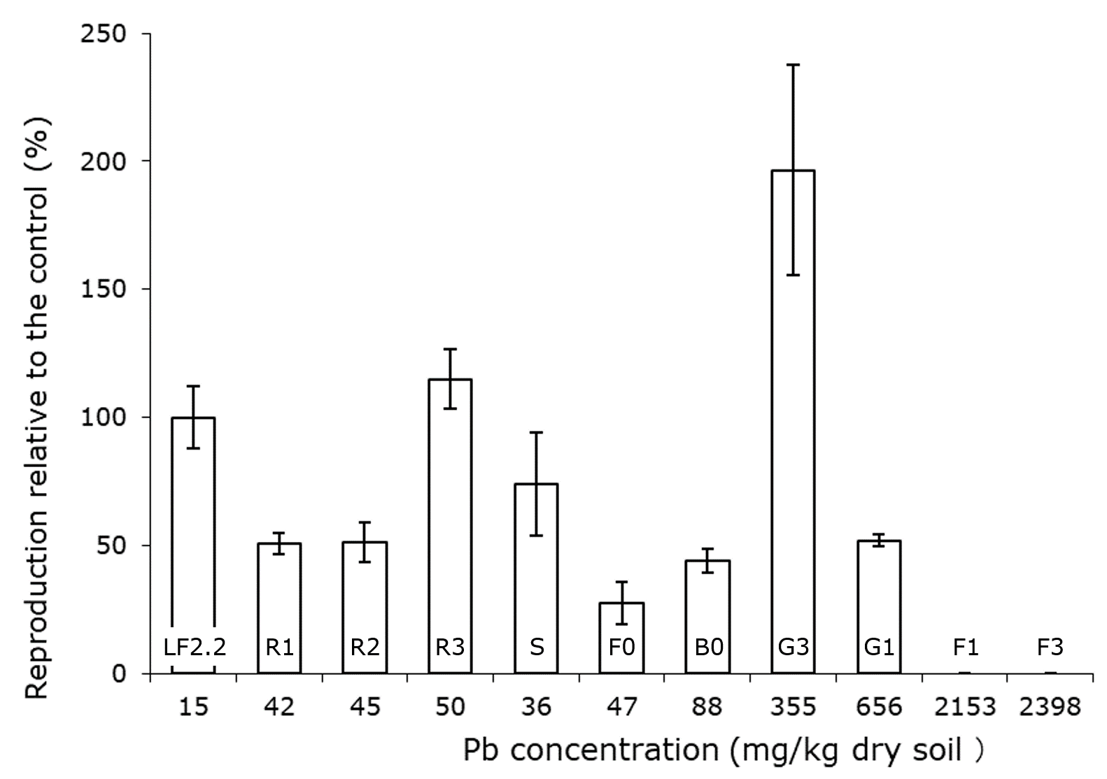
For the soil compartment, the earthworms Eisenia fetida, E. andrei and Lumbricus rubellus, the enchytraeid Enchytraeus crypticus and the collembolan Folsomia candida are most frequently selected as in vivo bioassay test organisms. An example of employing earthworms to assess the ecotoxicological effects of Pb contaminated soils is given in Figure 1. The figure shows the total Pb concentrations in different field soils taken from a soccer field (S), a bullet plot (B), grassland (G1, G3) and a forest (F1-F3) site near a shooting range. The pH of the grassland soils was near neutral (pHCaCl2 = 6.5-6.8), but the pH was rather low (3.2-3.7) for all other field sites. Earthworms exposed to these soils showed a significantly reduced reproductive output (Figure 1) at the most contaminated sites. At the less contaminated sites, earthworm responses were also affected by the difference in soil pH, leading to low juvenile numbers in the acid soil F0 but high numbers in the near neutral reference R3 and the field soil G3. In fact, earthworm reproduction was highest in the latter soil, even though it did contain an elevated concentration of 355 ± 54 mg Pb/kg dry soil. In soil G1, which contained almost twice as much Pb (656 ± 60 mg Pb/kg dry soil), reproduction was much lower and also reduced compared to the control, suggesting the presence of additional, unknown stressor (Luo et al., 2014).
For water, predominantly daphnids are employed, mainly Daphnia magna, but sometimes also other daphnid species or other aquatic invertebrates are selected. Also bioassays with several primary producers are available. An example of exposing daphnids (Chydorus sphaericus) to water samples is shown in Figure 2. The bars show the toxicity of the water samples and the diamonds the concentrations of cholinesterase inhibitors, as a proxy for the presence of insecticides. The toxicity of the water samples was higher when also the concentrations of insecticides were higher. Hence, in this case, the observed toxicity is well explained by the measured compounds. Yet, it has to be realized that this is an exception rather than a rule, since mostly a large portion of the toxic effects observed in surface waters cannot be attributed to compounds measured by water authorities and moreover, interactions are also not covered by such analytical data (see section on Effect based water quality assessment).

For sediments, oligochaetes and chironomids are selected as test organisms, but sometimes also rooting macrophytes and benthic diatoms. An example of exposing chironomids (Chironomus riparius) to contaminated sediments is shown in Figure 3. Whole sediment bioassays with chironomids allow the assessment of sensitive species-specific sublethal endpoints (see section on Chronic toxicity), in this case emergence. Figure 3 shows that more chironomids emerged on the reference sediment than on the contaminated sediment and that the chironomids on the reference sediment also emerged faster than on the contaminated sediment.

For sediment, also benthic diatoms are selected as in vivo bioassay test organisms. Figure 4 shows the growth of the benthic diatom Nitzschia perminuta after 4 days of exposure to 160 sediment samples. The dotted line represents control growth. The growth of the diatoms ranged from higher than the controls to no growth at all, raising the question which deviation from the control should be considered a significant adverse effect.

In vivo bioassay batteries
Environmental quality assessments are often performed with a single test species, like the four examples given above. Yet, toxicity is species and compound specific and this may therefore result in large margins of uncertainty in the environmental quality assessments, consequently leading to over- or underestimation of environmental risks. Obvious examples include the presence of herbicides that only would induce responses in bioassays with primary producers and the other way around, the presence of insecticides that induces strong effects on insects and to a lesser extent on other animals, but that would be completely overlooked in bioassays with primary producers. To reduce these uncertainties and to increase ecological relevance it is therefore advised to incorporate more test species belonging to different taxa in a bioassay battery (see section on Effect based water quality assessment).
References
Luo, W., Verweij, R.A., Van Gestel, C.A.M. (2014). Determining the bioavailability and toxicity of lead to earthworms in shooting range soils using a combination of physicochemical and biological assays. Environmental Pollution 185, 1-9.
Pieters, B.J., Bosman-Meijerman, D., Steenbergen, E., Van den Brandhof, E.-J., Van Beelen, P., Van der Grinten, E., Verweij, W., Kraak, M.H.S. (2008). Ecological quality assessment of Dutch surface waters using a new bioassay with the cladoceran Chydorus sphaericus. Proceedings Netherlands Entomological Society Meetings 19, 157-164.
Define in vivo bioassays and explain how in vivo bioassays are performed.
Give examples of the most commonly used in vivo bioassays per environmental compartment.
Motivate the necessity to incorporate several in vivo bioassays into a bioassay battery.
6.4.4. Effect Based water quality assessment
Effect-based water quality assessment
Authors: Milo de Baat, Michiel Kraak
Reviewers: Ad Ragas, Ron van der Oost, Beate Escher
Learning objectives:
You should be able to
- list the advantages and drawbacks of an effect-based monitoring approach in comparison to a compound-based approach for water quality assessment.
- motivate the necessity of employing a bioassay battery in effect-based monitoring approaches.
- explain the expression of bioassay responses in terms of toxic/bioanalytical equivalents of reference compounds.
- translate the outcome of a bioassay battery into a ranking of contaminated sites based on ecotoxicological risk.
Keywords: Effect-based monitoring, water quality assessment, bioassay battery, effect-based trigger values, ecotoxicological risk assessment
Introduction
Traditional chemical water quality assessment is based on the analysis of a list of a varying, but limited number of priority substances. Nowadays, the use of many of these compounds is restricted or banned, and concentrations of priority substances in surface waters are therefore decreasing. At the same time, industries have switched to a plethora of alternative compounds, which may enter the aquatic environment, seriously impacting water quality. Hence, priority substances lists are outdated, as the selected compounds are frequently absent, while many compounds with higher relevance are not listed as priority substances. Consequently, a large portion of toxic effects observed in surface waters cannot be attributed to compounds measured by water authorities, and toxic risks to freshwater ecosystems are thus caused by mixtures of a myriad of (un)known, unregulated compounds. Understanding of these risks requires a paradigm shift towards new monitoring methods that do not depend on chemical analysis of priority substances solely, but consider the biological effects of the entire micropollutant mixture first. Therefore, there is a need for effect-based monitoring strategies that employ bioassays to identify environmental risk. Responses in bioassays are caused by all bioavailable (un)known compounds and their metabolites, whether or not they are listed as priority substances.
Table 1. Example of the bioassay battery employed by the SIMONI approach of Van der Oost et al. (2017) that can be applied to assess surface water toxicity. Effect-based trigger values (EBT) were previously defined by Escher et al. (2018) (PAH, anti-AR and ER CALUX) and Van der Oost et al. (2017).
|
Bioassay |
Endpoint |
Reference compound |
EBT |
Unit |
|
|
in situ |
Daphnia in situ |
Mortality |
n/a |
20 |
% mortality |
|
in vivo |
Daphniatox |
Mortality |
n/a |
0.05 |
TU |
|
Algatox |
Algal growth inhibition |
n/a |
0.05 |
TU |
|
|
Microtox |
Luminescence inhibition |
n/a |
0.05 |
TU |
|
|
in vitro CALUX |
cytotox |
Cytotoxicity |
n/a |
0.05 |
TU |
|
DR |
Dioxin (-like) activity |
2,3,7,8-TCDD |
50 |
pg TEQ/L |
|
|
PAH |
PAH activity |
benzo(a)pyrene |
6.21 |
ng BapEQ/L |
|
|
PPARγ |
Lipid metabolism inhibition |
rosiglitazone |
10 |
ng RosEQ/L |
|
|
Nrf2 |
Oxidative stress |
curcumin |
10 |
µg CurEQ/L |
|
|
PXR |
Toxic compound metabolism |
nicardipine |
3 |
µg NicEQ/L |
|
|
p53 -S9 |
Genotoxicity |
n/a |
0.005 |
TU |
|
|
p53 +S9 |
Genotoxicity (after metabolism) |
n/a |
0.005 |
TU |
|
|
ER |
Estrogenic activity |
17ß-estradiol |
0.1 |
ng EEQ/L |
|
|
anti-AR |
Antiandrogenic activity |
flutamide |
14.4 |
µg FluEQ/L |
|
|
GR |
Glucocorticoid activity |
dexamethasone |
100 |
ng DexEQ/L |
|
|
in vitro antibiotics |
T |
Bacterial growth inhibition (Tetracyclines) |
oxytetracycline |
250 |
ng OxyEQ/L |
|
Q |
Bacterial growth inhibition (Quinolones) |
flumequine |
100 |
ng FlqEQ/L |
|
|
B+M |
Bacterial growth inhibition (β-lactams and Macrolides) |
penicillin G |
50 |
ng PenEQ/L |
|
|
S |
Bacterial growth inhibition (Sulfonamides) |
sulfamethoxazole |
100 |
ng SulEQ/L |
|
|
A |
Bacterial growth inhibition (Aminoglycosides) |
neomycin |
500 |
ng NeoEQ/L |
Bioassay battery
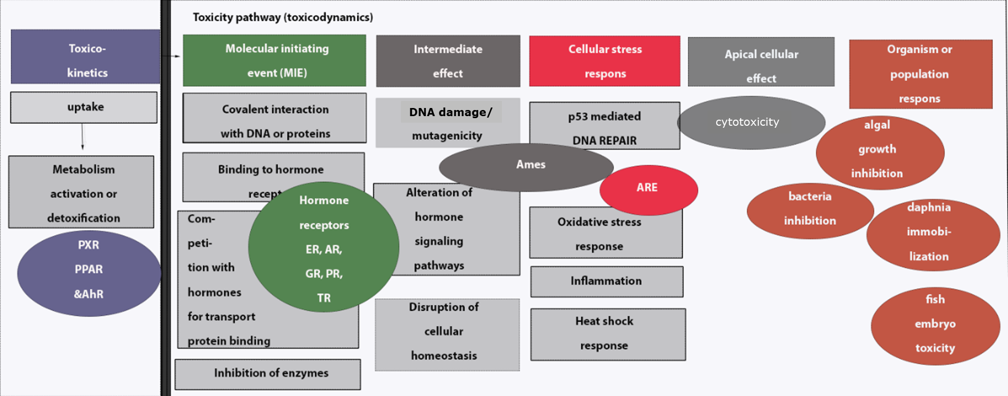
The regular application of effect-based monitoring largely relies on the ease of use, endpoint specificity, costs and size of the used bioassays, as well as on the ability to interpret the measured responses. To ensure sensitivity to a wide range of potential stressors, while still providing specific endpoint sensitivity, a successful bioassay battery like the example given in Table 1 can include in situ whole organism assays (see section on Biomonitoring and in situ bioassays), and should include laboratory-based whole-organism in vivo (see section on In vivo bioassays) and mechanism-specific in vitro assays (see section on In vitro bioassays). Adverse effects in the whole-organism bioassays point to general toxic pressure and represent a high ecological relevance. In vitro or small-scale in vivo assays with specific drivers of adverse effects allow for focused identification and subsequent confirmation of (groups of) toxic compounds with specific modes of action. Bioassay selection can also be based on the Adverse Outcome Pathways (AOP) (see section on Adverse Outcome Pathways) concept that describes relationships between molecular initiating events and adverse outcomes. Combining different types of bioassays ranging from whole organism tests to in vitro assays targeting specific modes of action can thus greatly aid in narrowing down the number of candidate compound(s) that cause environmental risks. For example, if bioanalytical responses at a higher organisational level are observed (the orange and black pathways in Figure 1), responses in specific molecular pathways (blue, green, grey and red in Figure 1) can help to identify certain (groups of) compounds responsible for the observed effects.
Toxic and bioanalytical equivalent concentrations
The severity of the adverse effect of an environmental sample in a bioassay is expressed as toxic equivalent (TEQ) concentrations for toxicity in in vivo assays or as bioanalytical equivalent (BEQ) concentrations for responses in in vitro bioassays. The toxic equivalent concentrations and bioanalytical equivalent concentrations represent the joint toxic potency of all unknown chemicals present in the sample that have the same mode of action (see section on Toxicodynamics and molecular interactions) as the reference compound and act concentration-additively (see section on Mixture toxicity). The toxic equivalent concentrations and bioanalytical equivalent concentrations are expressed as the concentration of a reference compound that causes an effect equal to the entire mixture of compounds present in an environmental sample. Figure 2 depicts a typical dose-response curve for a molecular in vitro assay that is indicative of the presence of compounds with a specific mode of action targeted by this in vitro assay. A specific water sample induced an effect of 38% in this assay, equivalent to the effect of approximately 0.02 nM bioanalytical equivalents.
Effect-based trigger values
The identification of ecological risks from bioassay battery responses follows from the comparison of bioanalytical signals to previously determined thresholds, defined as effect-based trigger values (EBT), that should differentiate between acceptable and poor water quality. Since bioassays potentially respond to the mixture of all compounds present in a sample, effect-based trigger values are expressed as toxic or bioanalytical equivalents of concentrations of model compounds for the respective bioassay (Table 1).

Ranking of contaminated sites based on effect-based risk assessment
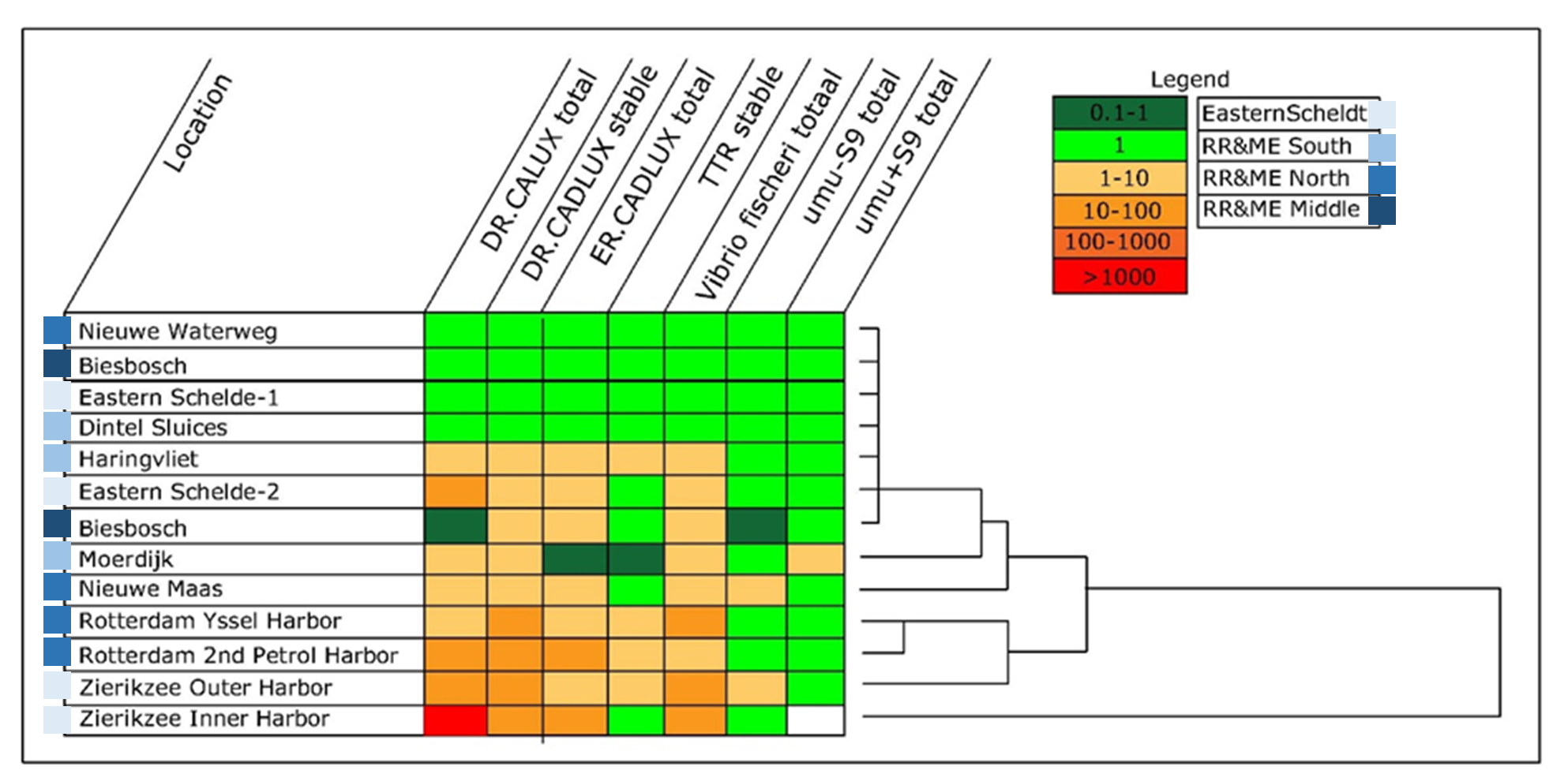
Once the toxic potency of a sample in a bioassay is expressed as toxic equivalent concentrations or bioanalytical equivalent concentrations, this response can be compared to the effect-based trigger value for that assay, thus determining whether or not there is a potential ecological risk from contaminants in the investigated water sample. The ecotoxicity profiles of the surface water samples generated by a bioassay battery allow for calculation and ranking of a cumulative ecological risk for the selected locations. In the example given in Figure 3, water samples of six locations were subjected to the SIMONI bioassay battery of Van der Oost et al. (2017), consisting of 17 in situ, in vivo and in vitro bioassays. Per site and per bioassay the response is compared to the corresponding effect-based trigger value and classified as 'no response' (green), 'response below the effect-based trigger value' (yellow) or 'response above the effect-based trigger value' (orange). Next, the cumulative ecological risk per location is calculated.
The resulting integrated ecological risk score allows ranking of the selected sites based on the presence of ecotoxicological risks rather than on the presence of a limited number of target compounds. This in turn permits water authorities to invest money where it matters most: identification of compounds causing adverse effects at locations with indicated ecotoxicological risks. Initially, the compounds causing the observed effect-based trigger value exceedance will not be known, however, this can subsequently be elucidated with targeted or non-target chemical analysis, which will only be necessary at locations with indicated ecological risks. A potential follow-up step could be to investigate the drivers of the observed effects by means of effect-directed analysis (see section on Effect-directed analysis).

References
Escher, B. I., Aїt-Aїssa, S., Behnisch, P. A., Brack, W., Brion, F., Brouwer, A., et al. (2018). Effect-based trigger values for in vitro and in vivo bioassays performed on surface water extracts supporting the environmental quality standards (EQS) of the European Water Framework Directive. Science of the Total Environment 628-629, 748-765.
Van der Oost, R., Sileno, G., Suarez-Munoz, M., Nguyen, M.T., Besselink, H., Brouwer, A. (2017). SIMONI (Smart Integrated Monitoring) as a novel bioanalytical strategy for water quality assessment: part I - Model design and effect-based trigger values. Environmental Toxicology and Chemistry 36, 2385-2399.
Additional reading
Altenburger, R., Ait-Aissa, S., Antczak, P., Backhaus, T., Barceló, D., Seiler, T.-B., et al. (2015). Future water quality monitoring - Adapting tools to deal with mixtures of pollutants in water resource management. Science of the Total Environment 512-513, 540-551.
Escher, B.I., Leusch, F.D.L. (2012). Bioanalytical Tools in Water Quality Assessment. IWA publishing, London (UK).
Hamers, T., Legradi, J., Zwart, N., Smedes, F., De Weert, J., Van den Brandhof, E-J., Van de Meent, D., De Zwart, D. (2018). Time-Integrative Passive sampling combined with TOxicity Profiling (TIPTOP): an effect-based strategy for cost-effective chemical water quality assessment. Environmental Toxicology and Pharmacology 64, 48-59.
List 5 advantages of an effect-based approach over a compound based approach for water quality assessment.
Motivate the necessity of employing a bioassay battery in effect based monitoring approaches.
Explain how bioassay responses are expressed in terms of toxicity equivalents of reference compounds? (you may wish to draw a figure).
Translate the outcome of a bioassay battery into a ranking of contaminated sites based on ecotoxicological risk. (you may wish to draw a figure).
6.4.5. Biomonitoring: in situ bioassays and contaminant concentrations in organisms
Author: Michiel Kraak
Reviewers: Ad Ragas, Suzanne Stuijfzand, Lieven Bervoets
Learning objectives:
You should be able to
- name tools specifically designed for ecological risk assessment in the field.
- define biomonitoring and to describe biomonitoring procedures.
- list the characteristics of suitable biomonitoring organisms.
- list the most commonly used biomonitoring organisms per environmental compartment.
- argue the advantages and disadvantages of in situ bioassays.
- argue the advantages and disadvantages of measuring contaminant concentrations in organisms.
Key words: Biomonitoring, test organisms, in situ bioassays, contaminant concentrations in organisms, environmental quality
Introduction
Several approaches and tools are available for diagnostic risk assessment. Tools specially developed for field assessments include the TRIAD approach (see section on TRIAD approach), in situ bioassays and biomonitoring. In ecotoxicology, biomonitoring is defined as the use of living organisms for the in situ assessment of environmental quality. Passive biomonitoring and active biomonitoring are distinguished. For passive biomonitoring, organisms are collected at the site of interest and their condition is assessed or the concentrations of specific target compounds in their tissues are analysed, or both. By comparing individuals from reference and contaminated sites an indication of the impact on local biota at the site of interest is obtained. For active biomonitoring, organisms are collected from reference sites and exposed in cages or artificial substrates at the study sites. Ideally, reference organisms are simultaneously exposed at the site of origin to control for potential effects of the experimental set-up on the test organisms. As an alternative to field collected animals, laboratory cultured organisms may be employed. After exposure at the study sites for a certain period of time, the organisms are recollected and either their condition is analysed (in situ bioassay) or the concentrations of specific target compounds are measured in the organisms, or both.
The results of biomonitoring studies may be used for management decisions, e.g. when accumulation of contaminants has been demonstrated in the field and especially when the sources of the pollution have been identified. However, the use of biomonitoring studies in environmental management has not been captured in formal protocols or guidelines like those of the Water Framework Directive (WFD) or - to a lesser extent - the TRIAD approach and effect-based quality assessments. Biomonitoring studies are typically applied on an case-by-case basis and their application therefore strongly depends on the expertise and resources available for the assessment. The text below explains and discusses the most important aspects of biomonitoring techniques used in diagnostic risk assessment.
Selection of biomonitoring test organisms
The selection of adequate organisms for biomonitoring partly follows the selection of test organisms for toxicity tests (see section on the Selection of test organisms). Suitable biomonitoring organisms:
- Are sedentary, since sedentary organisms may adapt more easily to the in situ experimental setup than more mobile organisms, for which caging may be an additional stress factor. Moreover, for sedentary organisms the relationship between the accumulated compounds and the environmental quality at the exposure site is straightforward, although this is more relevant to passive than to active biomonitoring.
- Are representative for the community of interest and native to the study sites, since this will ensure that the biomonitoring organisms tolerate local conditions other than contamination, preventing that stressors other than poor environmental conditions may affect their performance. Obviously, it is also undesirable to introduce exotic species into new environments.
- Are long living, at least substantially longer than the exposure duration and preferably large enough to obtain sufficient material for chemical analysis.
- Are easy to handle.
- Respond to a gradient of environmental quality, if the purpose of the biomonitoring study is to analyse the condition of the organisms after recollection (in situ bioassay).
- Accumulate contaminants without being killed, if the purpose of the biomonitoring study is to measure contaminant concentrations in the organisms after recollection.
- Are large enough to obtain sufficient biomass for the analysis of the target compounds above the limits of detection, if the purpose of the biomonitoring study is to measure contaminant concentrations in the organisms after recollection.
Based on the above listed criteria, in the marine environment mussels belonging to the genus Mytilus are predominantly selected. The genus Mytilus has the additional advantage of a global distribution, although represented by different species. This facilitates the comparison of contaminant concentrations in the organisms all around the globe. Lugworms have occasionally also been used for biomonitoring in marine systems. For freshwater, the cladoceran Daphnia magna is most frequently employed, although occasionally other species are selected, including mayflies, snails, worms, amphipods, isopods, caddisflies and fish. Given the positive experience with marine mussels, freshwater bivalves are also employed as biomonitoring organisms. Sometimes primary producers have been used, mainly periphyton. Due to the complexity of the sediment and soil compartments, few attempts have been made to expose organisms in situ, mainly restricted to chironomids on sediment.
In situ exposure devices
An obvious requirement of the in situ exposure devices is that the test organisms do not suffer from (sub)lethal effects of the experimental setup. If the organisms are large enough, cages may be used, like for freshwater and marine mussels. For daphnids, a simple glass jar with a permeable lid suffices. For riverine insects, the device should allow the natural flow of the stream to pass, but meanwhile prevent the organisms from escaping. In the device shown in Figure 1a, caddisfly larvae containing tubes are connected to floating tubes, maintaining the larvae at a constant depth of 65 cm. In the tubes, the caddisfly larvae are able to settle and build nets on artificial substrate, a plastic doormat with bristles standing out.
An elegant device for in situ colonization of periphyton was developed by Blanck (1985)(Figure 1b). Sand-blasted glass discs (1.5 cm2 surface) are used as artificial substratum for algal attachment. Substrata are placed vertically in the water, parallel to the current, by means of polyethylene racks, each rack supporting a total of 170 discs. After the colonization period, the periphyton containing glass discs can be harvested, offering the unique possibility to perform laboratory or field experiments with entire algal and microbial communities, replicated 170 times.

In situ bioassays
After exposure at the study sites for a certain period of time, the organisms are recollected and their condition can be analysed (Figure 2). The endpoint is mostly survival, especially in routine monitoring programs. If the in situ exposure lasts long enough, also effects on species specific sublethal endpoints can be assessed. For daphnids and snails, this is reproduction and for isopods growth. For aquatic insects (mayflies, caddisflies, damselflies, chironomids), emergence has been assessed as a sensitive ecological relevant endpoint (Barmentlo et al., 2018).

In situ bioassays come closest to the actual field situation. Organisms are directly exposed at the site of interest and respond to all joint stressors present. Yet, this is also the limitation of the approach. If organisms do respond it remains unknown what causes the observed adverse effects. This could be (the combination of) any natural or anthropogenic physical or chemical stress factor. In situ bioassays can therefore be best combined with laboratory bioassays (see section on Bioassays) and the analysis of physico-chemical parameters, conform the TRIAD approach (see section on TRIAD approach). If the adverse effects are also observed in the bioassays under controlled laboratory conditions, then poor water quality is most likely the cause. The water sample may then be subjected to suspected target analysis, non-target analysis or effect directed analysis (EDA). If adverse effects are observed in situ but not in the laboratory, then the presence of hazardous compounds is most likely not the cause. Instead, the effects may be attributable to e.g. low pH, low oxygen concentrations, high temperatures etc, which may be verified by physico-chemical analysis in the field.
Online biomonitoring
A specific application of in situ bioassays are the online systems for continuous water quality monitoring. In these systems, behaviour is generally the endpoint (see section on Endpoints). Organisms are exposed in a laboratory setting in situ (on shore or on a boat) in an experimental device to a continuous flow of surface water. If the water quality changes, the organisms respond by changing their behaviour. Above a certain threshold an alarm may go off and, for instance, the intake of surface water for drinking water preparation can be temporarily stopped.
Contaminant concentrations in organisms
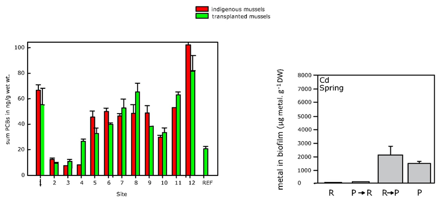
As an addition or as an alternative to analysing the condition of the exposed biomonitoring organisms upon retrieval, contaminant concentrations in organisms can be analysed. This has several advantages over chemical analysis of environmental samples: biomonitoring organisms may be exposed for days to weeks at the site of interest, providing time integrated measurements of contaminant concentrations, in contrast to the chemical analysis of grab samples. This way, biomonitoring organisms actually serve as 'biological passive samplers' (see to section on Experimental methods of assessing available concentrations of organic chemicals). Another advantage of measuring contaminant concentrations in organisms is that they only take up the bioavailable (fraction of) substances, ecologically very relevant information, that remains unknown if chemical analysis is performed on water, sediment, soil or air samples. Yet, elevated concentrations in organisms do not necessarily imply toxic effects, and therefore these measurements are best complemented with determining their condition, as described above. Moreover, analysing contaminants in organisms may be more expensive than measurements of environmental samples, due to a more complex sample preparation. Weighing the advantages and disadvantages, the explicit strength of biomonitoring programs is that they provide insight into the spatial and temporal variation in bioavailable contaminant concentrations. In Figure 3 two examples are given. The left panel shows the concentrations of PCBs in zebra mussels at different sampling sites in Flanders, Belgium (Bervoets et al., 2004). The right panel shows the rapid (within 2 wk) Cd accumulation and depuration in biofilms translocated from a reference to a polluted site and from a polluted to a reference site, respectively (Ivorra et al., 1999).
References
Barmentlo, S.H., Parmentier, E.M., De Snoo, G.R., Vijver, M.G. (2018). Thiacloprid-induced toxicity influenced by nutrients: evidence from in situ bioassays in experimental ditches. Environmental Toxicology and Chemistry 37, 1907-1915.
Bervoets, L., Voets, J., Chu, S.G., Covaci, A., Schepens, P., Blust, R. (2004). Comparison of accumulation of micropollutants between indigenous and transplanted zebra mussels (Dreissena polymorpha). Environmental Toxicology and Chemistry 23, 1973-1983.
Blanck, H. (1985). A simple, community level, ecotoxicological test systemusing samples of periphyton. Hydrobiologia 124, 251-261.
Ivorra, N., Hettelaar, J., Tubbing, G.M.J., Kraak, M.H.S., Sabater, S., Admiraal, W. (1999). Translocation of microbenthic algal assemblages used for in situ analysis of metal pollution in rivers. Archives of Environmental Contamination and Toxicology 37, 19-28.
Stuijfzand, S.C., Engels, S., Van Ammelrooy, E., Jonker, M. (1999). Caddisflies (Trichoptera: Hydropsychidae) used for evaluating water quality of large European rivers. Archives of Environmental Contamination and Toxicology 36, 186-192.
Vuori, K.M. (1995). Species- and population-specific responses of translocated hydropsychid larvae (Trichoptera, Hydropsychidae) to runoff from acid sulphate soils in the River Kyronjoki, western Finland. Freshwater Biology 33, 305-318.
Define biomonitoring.
Explain the difference between passive and active biomonitoring.
What can be measured in biomonitoring organisms after (re)collection?
Explain the difference between passive and active biomonitoring.
List the characteristics of suitable biomonitoring organisms.
Name the advantage and disadvantage of in situ bioassays.
Name the advantages and disadvantages of measuring contaminant concentrations in organisms.
6.4.6. TRIAD approach for site-specific ecological risk assessment
Author: Michiel Rutgers
Reviewers: Kees van Gestel, Michiel Kraak, Ad Ragas
Learning goals:
You should be able
- to describe the principles of the TRIAD approach
- to explain the importance of weight of evidence in risk assessment
- to use the results for an assessment by applying the TRIAD approach
Keywords: Triad, site-specific ecological risk assessment, weight of evidence
Like the other diagnostic tools described in the previous sections (see sections on Effect-based monitoring In vivo bioassays and In vitro bioassays, Effect-directed analysis, and Effect-based water quality assessment and Biomonitoring), the TRIAD approach is a tool for site-specific ecological risk assessment of contaminated sites (Jensen et al., 2006; Rutgers and Jensen, 2011). Yet, it differs from the previous approaches by combining and integrating different techniques through a 'weight of evidence' approach. To this purpose, the TRIAD combines information on contaminant concentrations (environmental chemistry), the toxicity of the mixture of chemicals present at the site ((eco)toxicology), and observations of ecological effects (ecology) (Figure 1).
The mere presence of contaminants is just an indication of potential ecological effects to occur. Additional data can help to better assess the ecological risks. For instance, information on actual toxicity of the contaminated site can be obtained from the exposure of test organisms to (extracts of) environmental samples (bioassays), while information on ecological effects can be obtained from an inventory of the community composition at the specific site. When these disciplines tend to converge to corresponding levels of ecological effects, a weight of evidence is established, making it possible to finalize the assessment and to support a decision for contaminated site management.

The TRIAD approach thus combines the information obtained from three lines of evidence (LoE):
- LoE Chemistry: risk information obtained from the measured contaminant concentrations and information on their fate in the ecosystem and how they can evoke ecotoxicological effects. This can include exposure modelling and bioavailability considerations.
- LoE Toxicity: risk information obtained from (eco)toxicity experiments exposing test organisms to (extracted) samples of the site. These bioassays can be performed on site or in the laboratory, under controlled conditions.
- LoE Ecology: risk information obtained from the observation of actual effects in the field. This is deduced from data of ecological field surveys, most often at the community level. This information may include data on the composition of soil communities or other community metrics and on ecosystem functioning.
The three lines of evidence form a weight of evidence when they are converging, meaning that when the independent lines of evidence are indicating a comparable risk level, there is sufficient evidence for providing advice to decision makers about the ecological risk at a contaminated site. When there is no convergence in risk information obtained from the three lines of evidence, uncertainty is large. Further investigations are then required to provide a unambiguous advice.
Table 1. Basic data for site-specific environmental risk assessment (SS-ERA) sorted per line of evidence (LoE). Data and methods are described in Van der Waarde et al. (2001) and Rutgers et al. (2001).
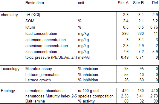
Tests and abbreviations used in the table:
- Toxic Pressure metals (sum TP metals). The toxic pressure of the mixture of metals in the sample, calculated as the potentially affected fraction in a Species Sensitivity Distribution with NOEC values (see Section on SSDs) and a simple rule for mixture toxicity (response addition; Section on Mixture toxicity).
- Microtox. A bioassay with the luminescent bacterium Allivibrio fischeri, formerly known as Vibrio fischeri. Luminescence is reduced when toxicity is high.
- Lettuce Growth and Lettuce Germination. A bioassay with the growth performance and the germination percentage of lettuce (seeds).
- Bait Lamina. The bait-lamina test consists of vertically inserting 16-hole-bearing plastic strips filled with a plant material preparation into the soil. This gives an indication of the feeding activity of soil animals.
- Nematodes abundance and Nematodes Maturity Index 2-5. The biomass and the Maturity Index (MI) of the nematode community in soil samples provide information about soil health (Van der Waarde et al. 2001).
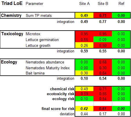
The results of a site-specific ecological risk assessment (SS-ERA) applying the TRIAD approach are first organized basic tables for each sample and line of evidence separately. Table 1 shows an example. This table also collects supporting data, such as soil pH and organic matter content. Subsequently, these basic data are processed into ecological risk values by applying a risk scale running from zero (no effects) to one (maximum effect). An example of a metric used is the multi-substance Potentially Affected Fraction of species from the mixture of contaminants (see Section on SSDs). These risk values are then collected in a TRIAD table (Table 2), for each endpoint separately, integrated per line of evidence individually, and finally integrated over the three lines of evidence. Also the level of agreement between the three lines of evidence is given a score. Weighting values are applied, e.g. equal weights for all ecological endpoints (depending on number of methods and endpoints), and equal weights for each line of evidence (33%). When differential weights are preferred, for instance when some data are judged as unreliable, or some endpoints are considered more important than others, the respective weight factors and the arguments to apply them must be provided in the same table and accompanying text.
Table 2. Soil Quality TRIAD table demonstrating scaled risk values for two contaminated sites (A, B) and a Reference site (based on real data, only for illustration purposes). Risk values are collected per endpoint, grouped according to respective Lines of Evidence (LoE), and finally integrated into a TRIAD value for risks. The deviation indicates a level of agreement between LoE (default threshold 0.4). For site B, a Weight of Evidence (WoE) is demonstrated (D<0.4) making decision support feasible. By default equal weights can be used throughout. Differential weights should be indicated in the table and described in the accompanying text.
References
ISO (2017). ISO 19204: Soil quality -- Procedure for site-specific ecological risk assessment of soil contamination (soil quality TRIAD approach). International Standardization Organization, Geneva. https://www.iso.org/standard/63989.html.
Jensen, J., Mesman, M. (Eds.) (2006). LIBERATION, Ecological risk assessment of contaminated land, decision support for site specific investigations. ISBN 90-6960-138-9, Report 711701047, RIVM, Bilthoven, The Netherlands.
Rutgers, M., Bogte, J.J., Dirven-Van Breemen, E.M., Schouten, A.J. (2001) Locatiespecifieke ecologische risicobeoordeling - praktijkonderzoek met een Triade-benadering. RIVM-rapport 711701026, Bilthoven.
Rutgers, M., Jensen, J. (2011). Site-specific ecological risk assessment. Chapter 15, in: F.A. Swartjes (Ed.), Dealing with Contaminated Sites - from Theory towards Practical Application, Springer, Dordrecht. pp. 693-720.
Van der Waarde, J.J., Derksen, J.G.M, Peekel, A.F., Keidel, H., Bloem, J., Siepel, H. (2001) Risicobeoordeling van bodemverontreiniging met behulp van een triade benadering met chemische analyses, bioassays en biologische veldinventarisaties. Eindrapportage NOBIS 98-1-28, Gouda.
A sediment sample was analyzed for Priority Hazardous Substances (PHSs), but none were detected. Yet, this sediment sample caused high mortality in laboratory bioassays with three sediment inhabiting species. At the site where the sample was taken biodiversity was very low. Explain these observations.
In a sediment sample, the total concentration of Priority Hazardous Substances (PHSs) was shown to be very high. Yet, this sediment sample caused no mortality in laboratory bioassays with three sediment inhabiting species. Moreover, at the sample site in the field species rich communities were observed. Explain these observations.
What is the added value of using bioassays and field observations over chemical analysis when assessing the potential risk of a contaminated site?
What is the added value of performing an assessment along three independent Lines of Evidence (LoE)?
6.4.7. Eco-epidemiology
Authors: Leo Posthuma, Dick de Zwart
Reviewers: Allan Burton, Ad Ragas
Learning objectives:
You should be able to:
- explain that and how effects of chemicals and their mixtures can be demonstrated in monitoring data sets;
- explain that effects can be characterized with various impact metrics;
- formulate whether and how the choice of impact sensitivity metric is relevant for the sensitivity and outcomes of a diagnostic assessment;
- explain how ecological and ecotoxicological analysis methods relate;
- explain how eco-epidemiological analyses are helpful in validating ecotoxicological models utilized in ecotoxicological risk assessment and management.
Keywords: eco-epidemiology, mixture pollution, diagnosis, impact magnitude, probable causes, validation
Introduction
Approaches for environmental protection, assessment and management differ between 'classical' stressors (such as excess nutrients and pH) and chemical pollution. For the 'classical' environmental stress factors, ecologists use monitoring data to develop concepts and methods to prevent and reduce impacts. Although there are some clear-cut examples of chemical pollution impacts [e.g., the decline in vulture populations in South East Asia due to diclofenac (Oaks et al. 2004), and the suit of examples in the book 'Silent Spring' (Carson 1962)], ecotoxicologists commonly have assessed the stress from chemical pollution by evaluating exposures vis a vis laboratory toxicity data. Current pollution often consists of complex mixtures of chemicals, with highly variable patterns in space and time. This poses problems when one wants to evaluate whether observed impacts in ecosystems can be attributed to chemicals or their mixtures. Eco-epidemiological methods have been established to discern such pollution stress. These methods provide the diagnostic tools to identify the impact magnitude and key chemicals that cause impacts in ecosystems. The use of these methods is further relevant for validating the laboratory-based risk assessment approaches developed by ecotoxicology.
The origins of eco-epidemiology
Risk assessments of chemicals provide insights in expected exposures and impacts, commonly for separate chemicals. These are predictive outcomes with a high relevance for decision making on environmental protection and management. The validation of those risk assessments is key to avoid wrong protection and management decisions, but it is complex. It consists of comparing predicted risk levels to observed effects. This begs the question on how to discern effects of chemical pollution in the field. This question can be answered based on the principles of ecological bio-assessments combined with those of human epidemiology. A bio-assessment is a study of stressors and ecosystem attributes, made to delineate causes of impacts via (often) statistical associations between biotic responses and particular stressors. Epidemiology is defined as the study of the distribution and causation of health and disease conditions in specified populations. Applied epidemiology serves as a scientific basis to help counteracting the spreading of human health problems. Dr. John Snow is often referred to as the 'father of epidemiology'. Based on observations on the incidence, locations and timings of the 1854 cholera outbreak in London, he attributed the disease to contaminated water taken from the Broad Street pump well, counteracting the prevailing idea that the disease was caused by transmission via air. His proposals to control the disease were effective. Likewise, eco-epidemiology - in its ecotoxicological context - has been defined as the study of the distribution and causation of impacts of multiple stressor exposures in ecosystems. In its applied form, it supports the reduction of ecological impacts of chemical pollution. Human-health eco-epidemiology is concerned with environment-mediated disease.
The first literature mention of eco-epidemiological analyses on chemical pollution stems from 1984 (Bro-Rasmussen and Løkke 1984). Those authors described eco-epidemiology as a discipline necessary to validate the risk assessment models and approaches of ecotoxicology. In its initial years, progress in eco-epidemiological research was slow due to practical constraints such as a lack of monitoring data, computational capacity and epidemiological techniques.
Current eco-epidemiology
Current eco-epidemiological studies in ecotoxicology aim to diagnose the impacts of chemical pollution in ecosystems, and utilize a combination of approaches in order to diagnose the role of chemical mixtures in causing ecological impacts in the field. The combination of approaches consists of:
1. Collection of monitoring data on abiotic characteristics and the occurrence and/or abundance of biotic species, for the environmental compartment under study;
2. If needed: data optimization, usually to align abiotic and biotic monitoring data, including the chemicals;
3. Statistical analysis of the data set using eco-epidemiological techniques to delineate impacts and probable causes, according to the approaches followed in 'classical' ecological bio-assessments;
4. Interpretation and use of the outcomes for either validation of ecotoxicological models and approaches, or for control of the impacts sensu Dr. Snow.
Key examples of chemical effects in nature
Although impacts of chemicals in the environment were known before 1962, Rachel Carson's book Silent Spring (see Section on the history of Environmental toxicology) can be seen as early and comprehensive eco-epidemiological study that synthesized the available information of impacts of chemicals in ecosystems. She considered effects of chemicals a novel force in natural selection when she wrote: "If Darwin were alive today the insect world would delight and astound him with its impressive verification of his theories of survival of the fittest. Under the stress of intensive chemical spraying the weaker members of the insect populations are being weeded out."
Clear examples of chemical impacts on species are still reported. Amongst the best-known examples is a study on vultures. The population of Indian vultures declined more than 95% due to diclofenac exposure which was used intensively as a veterinary drug (Oaks et al. 2004). The analysis of chemical impacts in nature becomes however more complex over time. The diversity of chemicals produced and used has vastly increased, and environmental samples contain thousands of chemicals at often low concentrations. Hence, contemporary eco-epidemiology is complex. Nonetheless, various studies demonstrated that contemporary mixture exposures affect species assemblages. Starting from large-scale monitoring data and following the four steps mentioned above, De Zwart et al. (2006) were able to show that effects on fish species assemblages could be attributed to both habitat characteristics and chemical mixtures. Kapo and Burton Jr (2006) showed the impacts of multiple stressors and chemical mixtures in aquatic species assemblages with similar types of data, but slightly different techniques. Eco-epidemiological studies of the effects of chemicals and their mixtures currently represent different geographies, species groups, stressors and chemicals/mixtures that are considered. The potential utility eco-epidemiological studies was reviewed by Posthuma et al. (2016). The review showed that mixture impacts occur, and that they can be separated from natural variability and multiple-stressor impacts. That means that water managers can develop management plans to counteract stressor impacts. Thereby, the study outcomes are used to prioritize management to sites that are most affected, and to chemicals that contribute most to those effects. Based on sophisticated statistical analyses, Berger et al. (2016) suggested chemicals can induce effects in the environment at concentrations much lower than expected based on laboratory experiments. Schäfer et al. (2016) argued that eco-epidemiological studies that cover both mixtures and other stressors are essential for environmental quality assessment and management. In practice, however, the analysis of the potential impacts of chemical mixtures is often still separate from the analysis of impacts of other stressors.
Steps in eco-epidemiological analysis
Various regulations require collection of monitoring data, followed by bio-assessment, such as the EU Water Framework Directive (see section on the Water Framework Directive). Therefore, monitoring data sets are increasingly available. The data set is subsequently curated and/or optimized for the analyses. Data curation and management steps imply amongst others that taxonomic names of species are harmonized, and that metrics for abiotic and biotic variables represent the conditions for the same place and time as much as possible. Next, the data set is expanded with novel variables, e.g. a metric for the toxic pressure exerted by chemical mixtures. An example of such a metric is the multi-substance Potentially Affected Fraction of species (msPAF). This metric transfers measured or predicted concentrations into the Potentially Affected Fraction of species (PAF), the values of which are then aggregated for a total mixture (De Zwart and Posthuma 2005). This is crucial, as adding each chemical of interest as a separate variable implies an increasingly expanding number of required sampling sites to maintain statistical power to diagnose impacts and probable causation.
The interpretation of the outcomes of the statistical analyses of the data set is the final step. Here, it must be acknowledged that statistical association is not equal to causation, and that care must be taken to explain the findings as indicative for mixture effects. Depending on the context of the study, this may then trigger a refined assessment, or alignment with other methods to collect evidence, or a direct use in an environmental management program.
Eco-epidemiological methods
A very basic eco-epidemiological method is quantile regression. Whereas common regression methods explore the magnitude of the change of the mean of the response variable (e.g., biodiversity) in relation to a predictor variable (e.g., pollutant stress), the quantile regression looks at the tails of the distributions of the response variable. How this principle operates is illustrated in Figure 1. When a monitoring data set contains one stressor variable at different levels (i.e., a gradient of data), the observations typically take the shape of a common stressor-response relationship (see section on Concentration-effect relationships). If the monitoring sites are affected by an extra stressor, the maximum-performance under the first stressor cannot be reached, so that the area under the curve contains the XY-points for this situation. Further addition of stressor variables and levels fills this space under the curve. When the raw data plotted as XY show an 'empty area' lacking XY-points, e.g. in the upper right corner, it is likely that the stressor variable can be identified as a stressor that limits the response variable, for example: chemicals limit biodiversity. The quantile regression calculates an upper percentiles (e.g., the 95th percentile) of the Y-values in assigned subgroups of X-values ("bins"). Such a procedure yields a picture such as Figure 1.

More complex methods for analysis of (bio)monitoring data have been developed and applied. The methods are closely associated to those developed for, and utilized in, applied ecology. Well-known examples are 'species distribution models' (SDM), which are used to describe the abundance or presence of species as a function of multiple environmental variables. A well-known SDM is the bell-shaped curve relating species abundances to water pH: numbers of individuals of a species are commonly low at low and high pH, and the SDM is characterized as an optimum model for species abundance (Y) versus pH (X). Statistical models can also describe species abundance, presence or biodiversity, as a function of multiple stressors, for example via Generalized Linear Models. These have the general shape of:
Log(Abundance)= (a. pH + a' pH2) + (b. OM + b' OM2) + …… + e,
with a, a', b and b' being estimated from fitting the model to the data, whilst pH and OM are the abiotic stressor variables (acidity and Organic Matter, respectively); the quadratic terms are added to allow for optimum and minimum shaped relationships. When SSD models (see Section on Species Sensitivity Distribution) are used to predict the multi-substance Potentially Affected Fraction of species, the resulting mixture stress proxy can be analysed together with the other stressor variables. Data analyses from monitoring data from the United States and the Netherlands have, for example, shown that the abundance of >60% of the taxa is co-affected by mixtures of chemicals. An example study is provided by Posthuma et al. (2016).
Prospective mixture impact assessments
In addition to the retrospective analysis of monitoring data, in search of chemical impacts, recent studies also show examples of prospective studies of effects of mixtures. Different land uses imply different chemical use patterns, summarized as 'signatures'. That is, agricultural land use will yield intermittent emissions of crop-specific plant protection products, aligning with the growing season. Emissions from populated areas will show continuous emission of household chemicals and discontinuous emissions of chemicals in street run-off associated to heavy rain events. The application of emission, fate and ecotoxicity models showed that aquatic ecosystems are subject to the 'signatures', with associated predicted impact magnitudes (Holmes et al. 2018; Posthuma et al. 2018). Although such prospective assessments did not yet prove ecological impacts, they can assist in avoiding impacts by preventing the emission 'signatures' that are identified as potentially most hazardous.
The use of eco-epidemiological output
Eco-epidemiological analysis outputs serve two purposes, closely related to prospective and retrospective risk assessment of chemical pollution:
1. Validation of ecotoxicological models and approaches;
2. Derivation of control measures, to reduce impacts of diagnosed probable causes of impacts.
If needed, multiple lines of evidence can be combined, such as in the Triad approach (see section on TRIAD) or approaches that consider more than three lines of evidence (Chapman and Hollert, 2006). The higher the importance of a good diagnosis, the better the user may rely on multiple lines of evidence.
First, the validation of ecotoxicological models and approaches is crucial, to avoid that important environmental protection, assessment and management activities rely on approaches that have limited relationship to field effects. Eco-epidemiological analyses have, for example, been used to validate the protective benchmarks used in the chemical-oriented environmental policies.
Second, the outcomes of an eco-epidemiological analysis can be used to control causes of impacts to ecosystems. Some studies have, for example, identified a statistical association between observed impacts (species expected but absent) and pollution of surface waters with mixtures of metals. Though local experts first doubted this association due to lack of industrial activities with metals in the area, they later found the association relevant given the presence of old spoil heaps from past mining activities. Metals appeared to leach into the surface waters at low rates, but the leached mixtures appeared to co-vary with species missing (De Zwart et al. 2006).
References
Berger, E., Haase, P., Oetken, M., Sundermann, A. (2016). Field data reveal low critical chemical concentrations for river benthic invertebrates. Science of The Total Environment 544, 864-873.
Bro-Rasmussen, F., Løkke, H. (1984). Ecoepidemiology - a casuistic discipline describing ecological disturbances and damages in relation to their specific causes; exemplified by chlorinated phenols and chlorophenoxy acids. Regulatory Toxicology and Pharmacology 4, 391-399.
Carson, R. (1962). Silent spring. Boston, Houghton Mifflin.
Chapman, P.M., Hollert, H. (2006). Should the sediment quality triad become a tetrad, a pentad, or possibly even a hexad? Journal of Soils and Sediments 6, 4-8.
De Zwart, D., Dyer, S.D., Posthuma, L., Hawkins, C.P. (2006). Predictive models attribute effects on fish assemblages to toxicity and habitat alteration. Ecological Applications 16, 1295-1310.
De Zwart, D., Dyer, S.D., Posthuma, L., Hawkins, C.P. (2006). Use of predictive models to attribute potential effects of mixture toxicity and habitat alteration on the biological condition of fish assemblages. Ecological Applications 16, 1295-1310.
De Zwart, D., Posthuma, L. (2005). Complex mixture toxicity for single and multiple species: Proposed methodologies. Environmental Toxicology and Chemistry 24,: 2665-2676.
Holmes, C.M., Brown, C.D., Hamer, M., Jones, R., Maltby, L., Posthuma, L., Silberhorn, E., Teeter, J.S., Warne, M.S.J., Weltje, L. (2018). Prospective aquatic risk assessment for chemical mixtures in agricultural landscapes. Environmental Toxicology and Chemistry 37, 674-689.
Kapo, K.E., Burton Jr, G.A. (2006). A geographic information systems-based, weights-of-evidence approach for diagnosing aquatic ecosystem impairment. Environmental Toxicology and Chemistry 25, 2237-2249.
Oaks, J.L., Gilbert, M., Virani, M.Z., Watson, R.T., Meteyer, C.U., Rideout, B.A., Shivaprasad, H.L., Ahmed, S., Chaudhry, M.J., Arshad, M., Mahmood, S., Ali, A., Khan, A.A. (2004). Diclofenac residues as the cause of vulture population decline in Pakistan. Nature 427(6975), 630-633.
Posthuma, L., Brown, C.D., de Zwart, D., Diamond, J., Dyer, S.D., Holmes, C.M., Marshall, S., Burton, G.A. (2018). Prospective mixture risk assessment and management prioritizations for river catchments with diverse land uses. Environmental Toxicology and Chemistry 37, 715-728.
Posthuma, L., De Zwart, D., Keijzers, R., Postma, J. (2016). Water systems analysis with the ecological key factor 'toxicity'. Part 2. Calibration. Toxic pressure and ecological effects on macrofauna in the Netherlands. Amersfoort, the Netherlands, STOWA.
Posthuma, L., Dyer, S.D., de Zwart, D., Kapo, K., Holmes, C.M., Burton Jr, G.A. (2016). Eco-epidemiology of aquatic ecosystems: Separating chemicals from multiple stressors. Science of The Total Environment 573, 1303-1319.
Posthuma, L., Suter, II, G.W., Traas, T.P. (Eds.) (2002). Species Sensitivity Distributions in Ecotoxicology. Boca Raton, FL, USA, Lewis Publishers.
Schäfer, R.B., Kühn, B., Malaj, E., König, A., Gergs, R. (2016). Contribution of organic toxicants to multiple stress in river ecosystems. Freshwater Biology 61, 2116-2128
Which motivations do you know for executing eco-epidemiological analyses?
Pollution in the 1950s and 1960s showed clear evidence for major impacts of chemicals in nature, whilst regulatory management actions taken since then have reduced clear recognition of chemical impacts in nature. Which ecotoxicological model has rejuvenated the development of eco-epidemiological methods?
What is a simple approach, via which even raw-data plottings already show whether a stress factor (such as chemical mixture exposure) is limiting for ecology