
8.4: Magnetic Force Microscopy
- Page ID
- 55920

\( \newcommand{\vecs}[1]{\overset { \scriptstyle \rightharpoonup} {\mathbf{#1}} } \)
\( \newcommand{\vecd}[1]{\overset{-\!-\!\rightharpoonup}{\vphantom{a}\smash {#1}}} \)
\( \newcommand{\id}{\mathrm{id}}\) \( \newcommand{\Span}{\mathrm{span}}\)
( \newcommand{\kernel}{\mathrm{null}\,}\) \( \newcommand{\range}{\mathrm{range}\,}\)
\( \newcommand{\RealPart}{\mathrm{Re}}\) \( \newcommand{\ImaginaryPart}{\mathrm{Im}}\)
\( \newcommand{\Argument}{\mathrm{Arg}}\) \( \newcommand{\norm}[1]{\| #1 \|}\)
\( \newcommand{\inner}[2]{\langle #1, #2 \rangle}\)
\( \newcommand{\Span}{\mathrm{span}}\)
\( \newcommand{\id}{\mathrm{id}}\)
\( \newcommand{\Span}{\mathrm{span}}\)
\( \newcommand{\kernel}{\mathrm{null}\,}\)
\( \newcommand{\range}{\mathrm{range}\,}\)
\( \newcommand{\RealPart}{\mathrm{Re}}\)
\( \newcommand{\ImaginaryPart}{\mathrm{Im}}\)
\( \newcommand{\Argument}{\mathrm{Arg}}\)
\( \newcommand{\norm}[1]{\| #1 \|}\)
\( \newcommand{\inner}[2]{\langle #1, #2 \rangle}\)
\( \newcommand{\Span}{\mathrm{span}}\) \( \newcommand{\AA}{\unicode[.8,0]{x212B}}\)
\( \newcommand{\vectorA}[1]{\vec{#1}} % arrow\)
\( \newcommand{\vectorAt}[1]{\vec{\text{#1}}} % arrow\)
\( \newcommand{\vectorB}[1]{\overset { \scriptstyle \rightharpoonup} {\mathbf{#1}} } \)
\( \newcommand{\vectorC}[1]{\textbf{#1}} \)
\( \newcommand{\vectorD}[1]{\overrightarrow{#1}} \)
\( \newcommand{\vectorDt}[1]{\overrightarrow{\text{#1}}} \)
\( \newcommand{\vectE}[1]{\overset{-\!-\!\rightharpoonup}{\vphantom{a}\smash{\mathbf {#1}}}} \)
\( \newcommand{\vecs}[1]{\overset { \scriptstyle \rightharpoonup} {\mathbf{#1}} } \)
\( \newcommand{\vecd}[1]{\overset{-\!-\!\rightharpoonup}{\vphantom{a}\smash {#1}}} \)
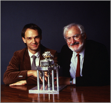
\(\newcommand{\avec}{\mathbf a}\) \(\newcommand{\bvec}{\mathbf b}\) \(\newcommand{\cvec}{\mathbf c}\) \(\newcommand{\dvec}{\mathbf d}\) \(\newcommand{\dtil}{\widetilde{\mathbf d}}\) \(\newcommand{\evec}{\mathbf e}\) \(\newcommand{\fvec}{\mathbf f}\) \(\newcommand{\nvec}{\mathbf n}\) \(\newcommand{\pvec}{\mathbf p}\) \(\newcommand{\qvec}{\mathbf q}\) \(\newcommand{\svec}{\mathbf s}\) \(\newcommand{\tvec}{\mathbf t}\) \(\newcommand{\uvec}{\mathbf u}\) \(\newcommand{\vvec}{\mathbf v}\) \(\newcommand{\wvec}{\mathbf w}\) \(\newcommand{\xvec}{\mathbf x}\) \(\newcommand{\yvec}{\mathbf y}\) \(\newcommand{\zvec}{\mathbf z}\) \(\newcommand{\rvec}{\mathbf r}\) \(\newcommand{\mvec}{\mathbf m}\) \(\newcommand{\zerovec}{\mathbf 0}\) \(\newcommand{\onevec}{\mathbf 1}\) \(\newcommand{\real}{\mathbb R}\) \(\newcommand{\twovec}[2]{\left[\begin{array}{r}#1 \\ #2 \end{array}\right]}\) \(\newcommand{\ctwovec}[2]{\left[\begin{array}{c}#1 \\ #2 \end{array}\right]}\) \(\newcommand{\threevec}[3]{\left[\begin{array}{r}#1 \\ #2 \\ #3 \end{array}\right]}\) \(\newcommand{\cthreevec}[3]{\left[\begin{array}{c}#1 \\ #2 \\ #3 \end{array}\right]}\) \(\newcommand{\fourvec}[4]{\left[\begin{array}{r}#1 \\ #2 \\ #3 \\ #4 \end{array}\right]}\) \(\newcommand{\cfourvec}[4]{\left[\begin{array}{c}#1 \\ #2 \\ #3 \\ #4 \end{array}\right]}\) \(\newcommand{\fivevec}[5]{\left[\begin{array}{r}#1 \\ #2 \\ #3 \\ #4 \\ #5 \\ \end{array}\right]}\) \(\newcommand{\cfivevec}[5]{\left[\begin{array}{c}#1 \\ #2 \\ #3 \\ #4 \\ #5 \\ \end{array}\right]}\) \(\newcommand{\mattwo}[4]{\left[\begin{array}{rr}#1 \amp #2 \\ #3 \amp #4 \\ \end{array}\right]}\) \(\newcommand{\laspan}[1]{\text{Span}\{#1\}}\) \(\newcommand{\bcal}{\cal B}\) \(\newcommand{\ccal}{\cal C}\) \(\newcommand{\scal}{\cal S}\) \(\newcommand{\wcal}{\cal W}\) \(\newcommand{\ecal}{\cal E}\) \(\newcommand{\coords}[2]{\left\{#1\right\}_{#2}}\) \(\newcommand{\gray}[1]{\color{gray}{#1}}\) \(\newcommand{\lgray}[1]{\color{lightgray}{#1}}\) \(\newcommand{\rank}{\operatorname{rank}}\) \(\newcommand{\row}{\text{Row}}\) \(\newcommand{\col}{\text{Col}}\) \(\renewcommand{\row}{\text{Row}}\) \(\newcommand{\nul}{\text{Nul}}\) \(\newcommand{\var}{\text{Var}}\) \(\newcommand{\corr}{\text{corr}}\) \(\newcommand{\len}[1]{\left|#1\right|}\) \(\newcommand{\bbar}{\overline{\bvec}}\) \(\newcommand{\bhat}{\widehat{\bvec}}\) \(\newcommand{\bperp}{\bvec^\perp}\) \(\newcommand{\xhat}{\widehat{\xvec}}\) \(\newcommand{\vhat}{\widehat{\vvec}}\) \(\newcommand{\uhat}{\widehat{\uvec}}\) \(\newcommand{\what}{\widehat{\wvec}}\) \(\newcommand{\Sighat}{\widehat{\Sigma}}\) \(\newcommand{\lt}{<}\) \(\newcommand{\gt}{>}\) \(\newcommand{\amp}{&}\) \(\definecolor{fillinmathshade}{gray}{0.9}\)Magnetic force microscopy (MFM) is a natural extension of scanning tunneling microscopy (STM), whereby both the physical topology of a sample surface and the magnetic topology may be seen. Scanning tunneling microscopy was developed in 1982 by Gerd Binnig and Heinrich Rohrer, and the two shared the 1986 Nobel prize for their innovation. Binnig later went on to develop the first atomic force microscope (AFM) along with Calvin Quate and Christoph Gerber (Figure \(\PageIndex{1}\)). Magnetic force microscopy was not far behind, with the first report of its use in 1987 by Yves Martin and H. Kumar Wickramasinge (Figure \(\PageIndex{2}\)). An AFM with a magnetic tip was used to perform these early experiments, which proved to be useful in imaging both static and dynamic magnetic fields.

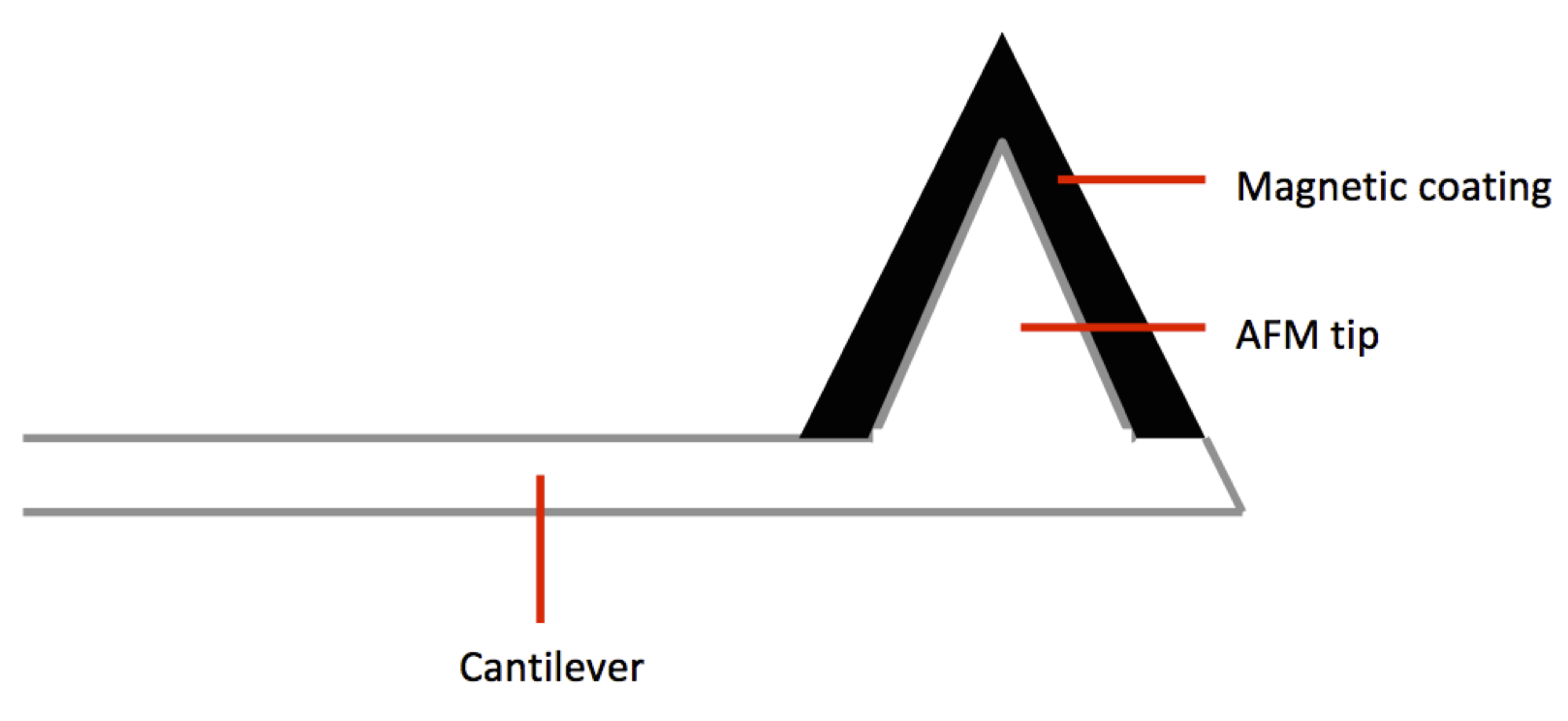
MFM, AFM, and STM all have similar instrumental setups, all of which are based on the early scanning tunneling microscopes. In essence, STM uses a very small conductive tip attached to a piezoelectric cylinder to carefully scan across a small sample space. The electrostatic forces between the conducting sample and tip are measured, and the output is a picture that shows the surface of the sample. AFM and MFM are essentially derivative types of STM, which explains why a typical MFM device is very similar to an STM, with a piezoelectric driver and magnetized tip as seen in Figure \(\PageIndex{3}\) and Figure \(\PageIndex{4}\).
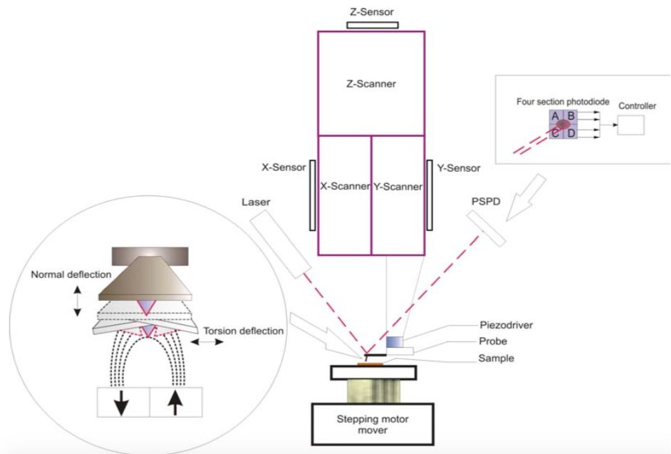
One may notice that this MFM instrument very closely resembles an atomic force microscope, and this is for good reason. The simplest MFM instruments are no more than AFM instruments with a magnetic tip. The differences between AFM and MFM lie in the data collected and its processing. Where AFM gives topological data through tapping, noncontact, or contact mode, MFM gives both topological (tapping) and magnetic topological (non-contact) data through a two-scan process known as interleave scanning. The relationships between basic STM, AFM, and MFM are summarized in Table \(\PageIndex{1}\).
| Techniques | Samples | Qualities Observed | Modes | Benefits | Limitations |
| MFM | Any film or powder surface; magnetic | Electrostatic interactions; magnetic forces/domains; van der Waals' interactions; topology; morphology | Tapping; non-contact | Magnetic and physical properties; high resolution | Resolution depends on tip size; different tips for various applications; complicated data processing and analysis |
| STM | Only conductive surfaces | Topology; morphology | Constant height; constant current | Simplest instrumental setup; many variations | Resolution depends on tip size; tips wear out easily; rare technique |
| AFM | Any film or powder surface | Particle size; topology; morphology | Tapping;contact; non-contact | Common, standardized; often do not need special tip; ease of data analysis | Resolution depends on tip size; easy to break tips; slow process |
Data Collection
Interleave scanning, also known as two-pass scanning, is a process typically used in an MFM experiment. The magnetized tip is first passed across the sample in tapping mode, similar to an AFM experiment, and this gives the surface topology of the sample. Then, a second scan is taken in non-contact mode, where the magnetic force exerted on the tip by the sample is measured. These two types of scans are shown in Figure \(\PageIndex{5}\).
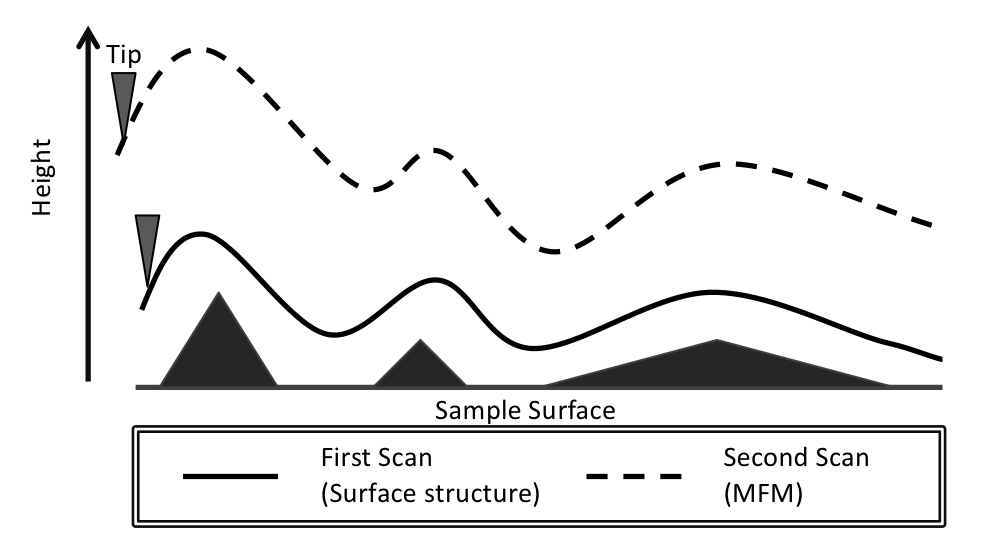
In non-contact mode (also called dynamic or AC mode), the magnetic force gradient from the sample affects the resonance frequency of the MFM cantilever, and can be measured in three different ways.
Phase detection: the phase difference between the oscillation of the cantilever and piezoelectric source is measured
Amplitude detection: the changes in the cantilever’s oscillations are measured
Frequency modulation: the piezoelectric source’s oscillation frequency is changed to maintain a 90° phase lag between the cantilever and the piezoelectric actuator. The frequency change needed for the lag is measured.
Regardless of the method used in determining the magnetic force gradient from the sample, a MFM interleave scan will always give the user information about both the surface and magnetic topology of the sample. A typical sample size is 100x100 μm, and the entire sample is scanned by rastering from one line to another. In this way, the MFM data processor can compose an image of the surface by combining lines of data from either the surface or magnetic scan. The output of an MFM scan is two images, one showing the surface and the other showing magnetic qualities of the sample. An idealized example is shown in Figure \(\PageIndex{6}\).

Types of MFM Tips
Any suitable magnetic material or coating can be used to make an MFM tip. Some of the most commonly used standard tips are coated with FeNi, CoCr, and NiP, while many research applications call for individualized tips such as carbon nanotubes. The resolution of the end image in MFM is dependent directly on the size of the tip, therefore MFM tips must come to a sharp point on the angstrom scale in order to function at high resolution. This leads to tips being costly, an issue exacerbated by the fact that coatings are often soft or brittle, leading to wear and tear. The best materials for MFM tips, therefore, depend on the desired resolution and application. For example, a high coercivity coating such as CoCr may be favored for analyzing bulk or strongly magnetic samples, whereas a low coercivity material such as FeNi might be preferred for more fine and sensitive applications.
Data Output and Applications
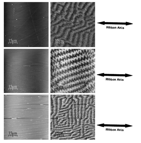
From an MFM scan, the product is a 2D scan of the sample surface, whether this be the physical or magnetic topographical image. Importantly, the resolution depends on the size of the tip of the probe; the smaller the probe, the higher the number of data points per square micrometer and therefore the resolution of the resulting image. MFM can be extremely useful in determining the properties of new materials, as in Figure \(\PageIndex{7}\), or in analyzing already known materials’ magnetic landscapes. This makes MFM particularly useful for the analysis of hard drives. As people store more and more information on magnetic storage devices, higher storage capacities need to be developed and emergency backup procedures for this data must be developed. MFM is an ideal procedure for characterizing the fine magnetic surfaces of hard drives for use in research and development, and also can show the magnetic surfaces of already-used hard drives for data recovery in the event of a hard drive malfunction. This is useful both in forensics and in researching new magnetic storage materials.
MFM has also found applications on the frontiers of research, most notably in the field of Spintronics. In general, Spintronics is the study of the spin and magnetic moment of solid-state materials, and the manipulation of these properties to create novel electronic devices. One example of this is quantum computing, which is promising as a fast and efficient alternative to traditional transistor-based computing. With regards to Spintronics, MFM can be used to characterize non-homogenous magnetic materials and unique samples such as dilute magnetic semiconductors (DMS). This is useful for research in magnetic storage such as MRAM, semiconductors , and magnetoresistive materials.
MFM for Characterization of Magnetic Storage Devices
In device manufacturing, the smoothness and/or roughness of the magnetic coatings of hard drive disks is significant in their ability to operate. Smoother coatings provide a low magnetic noise level, but stick to read/write heads, whereas rough surfaces have the opposite qualities. Therefore, fine tuning not only of the magnetic properties but the surface qualities of a given magnetic film is extremely important in the development of new hard drive technology. Magnetic force microscopy allows the manufacturers of hard drives to analyze disks for magnetic and surface topology, making it easier to control the quality of drives and determine which materials are suitable for further research. Industrial competition for higher bit density (bits per square millimeter), which means faster processing and increased storage capability, means that MFM is very important for characterizing films to very high resolution.
Conclusion
Magnetic force microscopy is a powerful surface technique used to deduce both the magnetic and surface topology of a given sample. In general, MFM offers high resolution, which depends on the size of the tip, and straightforward data once processed. The images outputted by the MFM raster scan are clear and show structural and magnetic features of a 100x100 μm square of the given sample. This information can be used not only to examine surface properties, morphology, and particle size, but also to determine the bit density of hard drives, features of magnetic computing materials, and identify exotic magnetic phenomena at the atomic level. As MFM evolves, thinner and thinner magnetic tips are being fabricated to finer applications, such as in the use of carbon nanotubes as tips to give high atomic resolution in MFM images. The customizability of magnetic coatings and tips, as well as the use of AFM equipment for MFM, make MFM an important technique in the electronics industry, making it possible to see magnetic domains and structures that otherwise would remain hidden.