
8.1: Microparticle Characterization via Confocal Microscopy
- Page ID
- 55917

\( \newcommand{\vecs}[1]{\overset { \scriptstyle \rightharpoonup} {\mathbf{#1}} } \)
\( \newcommand{\vecd}[1]{\overset{-\!-\!\rightharpoonup}{\vphantom{a}\smash {#1}}} \)
\( \newcommand{\id}{\mathrm{id}}\) \( \newcommand{\Span}{\mathrm{span}}\)
( \newcommand{\kernel}{\mathrm{null}\,}\) \( \newcommand{\range}{\mathrm{range}\,}\)
\( \newcommand{\RealPart}{\mathrm{Re}}\) \( \newcommand{\ImaginaryPart}{\mathrm{Im}}\)
\( \newcommand{\Argument}{\mathrm{Arg}}\) \( \newcommand{\norm}[1]{\| #1 \|}\)
\( \newcommand{\inner}[2]{\langle #1, #2 \rangle}\)
\( \newcommand{\Span}{\mathrm{span}}\)
\( \newcommand{\id}{\mathrm{id}}\)
\( \newcommand{\Span}{\mathrm{span}}\)
\( \newcommand{\kernel}{\mathrm{null}\,}\)
\( \newcommand{\range}{\mathrm{range}\,}\)
\( \newcommand{\RealPart}{\mathrm{Re}}\)
\( \newcommand{\ImaginaryPart}{\mathrm{Im}}\)
\( \newcommand{\Argument}{\mathrm{Arg}}\)
\( \newcommand{\norm}[1]{\| #1 \|}\)
\( \newcommand{\inner}[2]{\langle #1, #2 \rangle}\)
\( \newcommand{\Span}{\mathrm{span}}\) \( \newcommand{\AA}{\unicode[.8,0]{x212B}}\)
\( \newcommand{\vectorA}[1]{\vec{#1}} % arrow\)
\( \newcommand{\vectorAt}[1]{\vec{\text{#1}}} % arrow\)
\( \newcommand{\vectorB}[1]{\overset { \scriptstyle \rightharpoonup} {\mathbf{#1}} } \)
\( \newcommand{\vectorC}[1]{\textbf{#1}} \)
\( \newcommand{\vectorD}[1]{\overrightarrow{#1}} \)
\( \newcommand{\vectorDt}[1]{\overrightarrow{\text{#1}}} \)
\( \newcommand{\vectE}[1]{\overset{-\!-\!\rightharpoonup}{\vphantom{a}\smash{\mathbf {#1}}}} \)
\( \newcommand{\vecs}[1]{\overset { \scriptstyle \rightharpoonup} {\mathbf{#1}} } \)
\( \newcommand{\vecd}[1]{\overset{-\!-\!\rightharpoonup}{\vphantom{a}\smash {#1}}} \)
\(\newcommand{\avec}{\mathbf a}\) \(\newcommand{\bvec}{\mathbf b}\) \(\newcommand{\cvec}{\mathbf c}\) \(\newcommand{\dvec}{\mathbf d}\) \(\newcommand{\dtil}{\widetilde{\mathbf d}}\) \(\newcommand{\evec}{\mathbf e}\) \(\newcommand{\fvec}{\mathbf f}\) \(\newcommand{\nvec}{\mathbf n}\) \(\newcommand{\pvec}{\mathbf p}\) \(\newcommand{\qvec}{\mathbf q}\) \(\newcommand{\svec}{\mathbf s}\) \(\newcommand{\tvec}{\mathbf t}\) \(\newcommand{\uvec}{\mathbf u}\) \(\newcommand{\vvec}{\mathbf v}\) \(\newcommand{\wvec}{\mathbf w}\) \(\newcommand{\xvec}{\mathbf x}\) \(\newcommand{\yvec}{\mathbf y}\) \(\newcommand{\zvec}{\mathbf z}\) \(\newcommand{\rvec}{\mathbf r}\) \(\newcommand{\mvec}{\mathbf m}\) \(\newcommand{\zerovec}{\mathbf 0}\) \(\newcommand{\onevec}{\mathbf 1}\) \(\newcommand{\real}{\mathbb R}\) \(\newcommand{\twovec}[2]{\left[\begin{array}{r}#1 \\ #2 \end{array}\right]}\) \(\newcommand{\ctwovec}[2]{\left[\begin{array}{c}#1 \\ #2 \end{array}\right]}\) \(\newcommand{\threevec}[3]{\left[\begin{array}{r}#1 \\ #2 \\ #3 \end{array}\right]}\) \(\newcommand{\cthreevec}[3]{\left[\begin{array}{c}#1 \\ #2 \\ #3 \end{array}\right]}\) \(\newcommand{\fourvec}[4]{\left[\begin{array}{r}#1 \\ #2 \\ #3 \\ #4 \end{array}\right]}\) \(\newcommand{\cfourvec}[4]{\left[\begin{array}{c}#1 \\ #2 \\ #3 \\ #4 \end{array}\right]}\) \(\newcommand{\fivevec}[5]{\left[\begin{array}{r}#1 \\ #2 \\ #3 \\ #4 \\ #5 \\ \end{array}\right]}\) \(\newcommand{\cfivevec}[5]{\left[\begin{array}{c}#1 \\ #2 \\ #3 \\ #4 \\ #5 \\ \end{array}\right]}\) \(\newcommand{\mattwo}[4]{\left[\begin{array}{rr}#1 \amp #2 \\ #3 \amp #4 \\ \end{array}\right]}\) \(\newcommand{\laspan}[1]{\text{Span}\{#1\}}\) \(\newcommand{\bcal}{\cal B}\) \(\newcommand{\ccal}{\cal C}\) \(\newcommand{\scal}{\cal S}\) \(\newcommand{\wcal}{\cal W}\) \(\newcommand{\ecal}{\cal E}\) \(\newcommand{\coords}[2]{\left\{#1\right\}_{#2}}\) \(\newcommand{\gray}[1]{\color{gray}{#1}}\) \(\newcommand{\lgray}[1]{\color{lightgray}{#1}}\) \(\newcommand{\rank}{\operatorname{rank}}\) \(\newcommand{\row}{\text{Row}}\) \(\newcommand{\col}{\text{Col}}\) \(\renewcommand{\row}{\text{Row}}\) \(\newcommand{\nul}{\text{Nul}}\) \(\newcommand{\var}{\text{Var}}\) \(\newcommand{\corr}{\text{corr}}\) \(\newcommand{\len}[1]{\left|#1\right|}\) \(\newcommand{\bbar}{\overline{\bvec}}\) \(\newcommand{\bhat}{\widehat{\bvec}}\) \(\newcommand{\bperp}{\bvec^\perp}\) \(\newcommand{\xhat}{\widehat{\xvec}}\) \(\newcommand{\vhat}{\widehat{\vvec}}\) \(\newcommand{\uhat}{\widehat{\uvec}}\) \(\newcommand{\what}{\widehat{\wvec}}\) \(\newcommand{\Sighat}{\widehat{\Sigma}}\) \(\newcommand{\lt}{<}\) \(\newcommand{\gt}{>}\) \(\newcommand{\amp}{&}\) \(\definecolor{fillinmathshade}{gray}{0.9}\)A Brief History of Confocal Microscopy
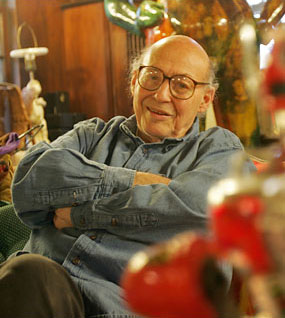
Confocal microscopy was invented by Marvin Minsky (FIGURE) in 1957, and subsequently patented in 1961. Minsky was trying to study neural networks to understand how brains learn, and needed a way to image these connections in their natural state (in three dimensions). He invented the confocal microscope in 1955, but its utility was not fully realized until technology could catch up. In 1973 Egger published the first recognizable cells, and the first commercial microscopes were produced in 1987.
In the 1990's confocal microscopy became near routine due to advances in laser technology, fiber optics, photodetectors, thin film dielectric coatings, computer processors, data storage, displays, and fluorophores. Today, confocal microscopy is widely used in life sciences to study cells and tissues.
The Basics of Fluorescence
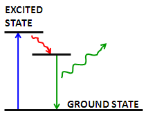
Fluorescence is the emission of a secondary photon upon absorption of a photon of higher wavelength. Most molecules at normal temperatures are at the lowest energy state, the so-called 'ground state'. Occasionally, a molecule may absorb a photon and increase its energy to the excited state. From here it can very quickly transfer some of that energy to other molecules through collisions; however, if it cannot transfer enough energy it spontaneously emits a photon with a lower wavelength Figure \(\PageIndex{2}\). This is fluorescence.
In fluorescence microscopy, fluorescent molecules are designed to attach to specific parts of a sample, thus identifying them when imaged. Multiple fluorophores can be used to simultaneously identify different parts of a sample. There are two options when using multiple fluorophores:
Fluorophores can be chosen that respond to different wavelengths of a multi-line laser.
Fluorophores can be chosen that respond to the same excitation wavelength but emit at different wavelengths.
In order to increase the signal, more fluorophores can be attached to a sample. However, there is a limit, as high fluorophore concentrations result in them quenching each other, and too many fluorophores near the surface of the sample may absorb enough light to limit the light available to the rest of the sample. While the intensity of incident radiation can be increased, fluorophores may become saturated if the intensity is too high.
Photobleaching is another consideration in fluorescent microscopy. Fluorophores irreversibly fade when exposed to excitation light. This may be due to reaction of the molecules’ excited state with oxygen or oxygen radicals. There has been some success in limiting photobleaching by reducing the oxygen available or by using free-radical scavengers. Some fluorophores are more robust than others, so choice of fluorophore is very important. Fluorophores today are available that emit photons with wavelengths ranging 400 - 750 nm.
How Confocal Microscopy is Different from Optical Microscopy
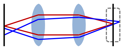
A microscope’s lenses project the sample plane onto an image plane. An image can be formed at many image planes; however, we only consider one of these planes to be the ‘focal plane’ (when the sample image is in focus). When a pinhole screen in placed at the image focal point, it allows in-focus light to pass while effectively blocking light from out-of-focus locations Figure \(\PageIndex{3}\). This pinhole is placed at the conjugate image plane to the focal plane, thus the name "confocal". The size of this pinhole determines the depth-of-focus; a bigger pinhole collects light from a larger volume. The pinhole can only practically be made as small as approximately the radius of the Airy disk, which is the best possible light spot from a circular aperture Figure \(\PageIndex{4}\), because beyond that more signal is blocked resulting in a decreased signal-to-boise ratio.
In optics, the Airy disk and Airy pattern are descriptions of the best focused spot of light that a perfect lens with a circular aperture can make, limited by the diffraction of light.

To further reduce the effect of scattering due to light from other parts of the sample, the sample is only illuminated at a tiny point through the use of a pinhole in front of the light source. This greatly reduces the interference of scattered light from other parts of the sample. The combination of a pinhole in front of both the light source and detector is what makes confocal unique.
Parts of a Confocal Microscope
A simple confocal microscope generally consists of a laser, pinhole aperture, dichromatic mirror, scanning mirrors, microscope objectives, a photomultiplier tube, and computing software used to reconstruct the image Figure \(\PageIndex{5}\). Because a relatively small volume of the sample is being illuminated at any given time, a very bright light source must be used to produce a detectable signal. Early confocal microscopes used zirconium arc lamps, but recent advances in laser technology have made lasers in the UV-visible and infrared more stable and affordable. A laser allows for a monochromatic (narrow wavelength range) light source that can be used to selectively excite fluorophores to emit photons of a different wavelength. Sometimes filters are used to further screen for single wavelengths.
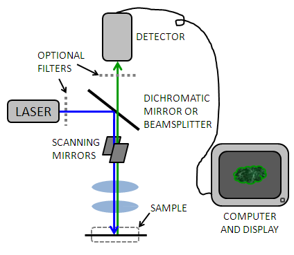
The light passes through a dichromatic (or "dichroic") mirror Figure \(\PageIndex{6}\) which allows light with a higher wavelength (from the laser) to pass but reflects light of a lower wavelength (from the sample) to the detector. This allows the light to travel the same path through the majority of the instrument, and eliminates signal due to reflection of the incident light.
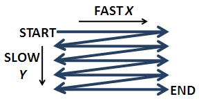
The light is then reflects across a pair of mirrors or crystals, one each for the x and y directions, which enable the beam to scan across the sample (Figure \(\PageIndex{6}\)). The speed of the scan is usually the limiting factor in the speed of image acquisition. Most confocal microscopes can create an image in 0.1 - 1 second. Usually the sample is raster scanned quickly in the x-direction and slowly in the y direction (like reading a paragraph left to right, Figure \(\PageIndex{6}\)).
The rastering is controlled by galvanometers that move the mirrors back and forth in a sawtooth motion. The disadvantage to scanning with the light beam is that the angle of light hitting the sample changes. Fortunately, this change is small. Interestingly, Minsky's original design moved the stage instead of the beam, as it was difficult to maintain alignment of the sensitive optics. Despite the obvious disadvantages of moving a bulky specimen, there are some advantages of moving the stage and keeping the optics stationary:
The light illuminates the specimen axially everywhere circumventing optical aberrations, and
The field of view can be made much larger by controlling the amplitude of the stage movements.
An alternative to light-reflecting mirrors is the acousto-optic deflector (AOD). The AOD allows for fast x-direction scans by creating a diffraction grating from high-frequency standing sound (pressure) waves which locally change the refractive index of a crystal. The disadvantage to AODs is that the amount of deflection depends on the wavelength, so the emission light cannot be descanned (travel back through the same path as the excitation light). The solution to this is to descan only in the y direction controlled by the slow galvanometer and collect the light in a slit instead of a pinhole. This results in reduced optical sectioning and slight distortion due to the loss of radial symmetry, but good images can still be formed. Keep in mind this is not a problem for reflected light microscopy which has the same wavelength for incident and reflected light!
Another alternative is the Nipkow disk, which has a spiral array of pinholes that create the simultaneous sampling of many points in the sample. A single rotation covers the entire specimen several times over (at 40 revolutions per second, that's over 600 frames per second). This allows descanning, but only about 1% of the excitation light passes through. This is okay for reflected light microscopy, but the signal is relatively weak and signal-to-noise ratio is low. The pinholes could be made bigger to increase light transmission but then the optical sectioning is less effective (remember depth of field is dependent on the diameter of the pinhole) and xy resolution is poorer. Highly responsive, efficient fluorophores are needed with this method.
Returning to the confocal microscope (Figure \(\PageIndex{5}\)), light then passes through the objective which acts as a well-corrected condenser and objective combination. The illuminated fluorophores fluoresce and emitted light travels up the objective back to the dichromatic mirror. This is known as epifluorescence when the incident light has the same path as detected light. Since the emitted light now has a lower wavelength than the incident, it cannot pass through the dichromatic mirror and is reflected to the detector. When using reflected light, a beamsplitter is used instead of a dichromatic mirror. Fluorescence microscopy when used properly can be more sensitive than reflected light microscopy.
Though the signal’s position is well-defined according to the position of the xy mirrors, the signal from fluorescence is relatively weak after passing through the pinhole, so a photomultiplier tube is used to detect emitted photons. Detecting all photons without regard to spatial position increases the signal, and the photomultiplier tube further increases the detection signal by propagating an electron cascade resulting from the photoelectric effect (incident photons kicking off electrons). The resulting signal is an analog electrical signal with continuously varying voltage that corresponds to the emission intensity. This is periodically sampled by an analog-to-digital converter.
It is important to understand that the image is a reconstruction of many points sampled across the specimen. At any given time the microscope is only looking at a tiny point, and no complete image exists that can be viewed at an instantaneous point in time. Software is used to recombine these points to form an image plane, and combine image planes to form a 3-D representation of the sample volume.
Two-photon Microscopy
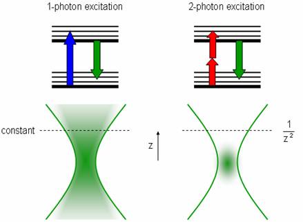
Two-photon microscopy is a technique whereby two beams of lower intensity are directed to intersect at the focal point. Two photons can excite a fluorophore if they hit it at the same time, but alone they do not have enough energy to excite any molecules. The probability of two photons hitting a fluorophore at nearly the exact same time (less than 10-16) is very low, but more likely at the focal point. This creates a bright point of light in the sample without the usual cone of light above and below the focal plane, since there are almost no excitations away from the focal point.
To increase the chance of absorption, an ultra-fast pulsed laser is used to create quick, intense light pulses. Since the hourglass shape is replaced by a point source, the pinhole near the detector (used to reduce the signal from light originating from outside the focal plane) can be eliminated. This also increases the signal-to-noise ratio (here is very little noise now that the light source is so focused, but the signal is also small). These lasers have lower average incident power than normal lasers, which helps reduce damage to the surrounding specimen. This technique can image deeper into the specimen (~400 μm), but these lasers are still very expensive, difficult to set up, require a stronger power supply, intensive cooling, and must be aligned in the same optical table because pulses can be distorted in optical fibers.
Microparticle Characterization
Confocal microscopy is very useful for determining the relative positions of particles in three dimensions Figure \(\PageIndex{8}\). Software allows measurement of distances in the 3D reconstructions so that information about spacing can be ascertained (such as packing density, porosity, long range order or alignment, etc.).
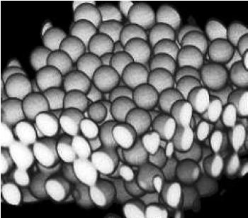
FIgure \(\PageIndex{8}\) A reconstruction of a colloidal suspension of poly(methyl methacrylate) (PMMA) microparticles approximately 2 microns in diameter. Adapted from Confocal Microscopy of Colloids, Eric Weeks.
If imaging in fluorescence mode, remember that the signal will only represent the locations of the individual fluorophores. There is no guarantee fluorophores will completely attach to the structures of interest or that there will not be stray fluorophores away from those structures. For microparticles it is often possible to attach the fluorophores to the shell of the particle, creating hollow spheres of fluorophores. It is possible to tell if a sample sphere is hollow or solid but it would depend on the transparency of the material.
Dispersions of microparticles have been used to study nucleation and crystal growth, since colloids are much larger than atoms and can be imaged in real-time. Crystalline regions are determined from the order of spheres arranged in a lattice, and regions can be distinguished from one another by noting lattice defects.
Self-assembly is another application where time-dependent, 3-D studies can help elucidate the assembly process and determine the position of various structures or materials. Because confocal is popular for biological specimens, the position of nanoparticles such as quantum dots in a cell or tissue can be observed. This can be useful for determining toxicity, drug-delivery effectiveness, diffusion limitations, etc.
A Summary of Confocal Microscopy's Strengths and Weaknesses
Strengths
Less haze, better contrast than ordinary microscopes.
3-D capability.
Illuminates a small volume.
Excludes most of the light from the sample not in the focal plane.
Depth of field may be adjusted with pinhole size.
Has both reflected light and fluorescence modes.
Can image living cells and tissues.
Fluorescence microscopy can identify several different structures simultaneously.
Accommodates samples with thickness up to 100 μm.
Can use with two-photon microscopy.
Allows for optical sectioning (no artifacts from physical sectioning) 0.5 - 1.5 μm.
Weaknesses
Images are scanned slowly (one complete image every 0.1-1 second).
Must raster scan sample, no complete image exists at any given time.
There is an inherent resolution limit because of diffraction (based on numerical aperture, ~200 nm).
Sample should be relatively transparent for good signal.
High fluorescence concentrations can quench the fluorescent signal.
Fluorophores irreversibly photobleach.
Lasers are expensive.
Angle of incident light changes slightly, introducing slight distortion.