
4.5: Photoluminescence, Phosphorescence, and Fluorescence Spectroscopy
- Page ID
- 55883

\( \newcommand{\vecs}[1]{\overset { \scriptstyle \rightharpoonup} {\mathbf{#1}} } \)
\( \newcommand{\vecd}[1]{\overset{-\!-\!\rightharpoonup}{\vphantom{a}\smash {#1}}} \)
\( \newcommand{\id}{\mathrm{id}}\) \( \newcommand{\Span}{\mathrm{span}}\)
( \newcommand{\kernel}{\mathrm{null}\,}\) \( \newcommand{\range}{\mathrm{range}\,}\)
\( \newcommand{\RealPart}{\mathrm{Re}}\) \( \newcommand{\ImaginaryPart}{\mathrm{Im}}\)
\( \newcommand{\Argument}{\mathrm{Arg}}\) \( \newcommand{\norm}[1]{\| #1 \|}\)
\( \newcommand{\inner}[2]{\langle #1, #2 \rangle}\)
\( \newcommand{\Span}{\mathrm{span}}\)
\( \newcommand{\id}{\mathrm{id}}\)
\( \newcommand{\Span}{\mathrm{span}}\)
\( \newcommand{\kernel}{\mathrm{null}\,}\)
\( \newcommand{\range}{\mathrm{range}\,}\)
\( \newcommand{\RealPart}{\mathrm{Re}}\)
\( \newcommand{\ImaginaryPart}{\mathrm{Im}}\)
\( \newcommand{\Argument}{\mathrm{Arg}}\)
\( \newcommand{\norm}[1]{\| #1 \|}\)
\( \newcommand{\inner}[2]{\langle #1, #2 \rangle}\)
\( \newcommand{\Span}{\mathrm{span}}\) \( \newcommand{\AA}{\unicode[.8,0]{x212B}}\)
\( \newcommand{\vectorA}[1]{\vec{#1}} % arrow\)
\( \newcommand{\vectorAt}[1]{\vec{\text{#1}}} % arrow\)
\( \newcommand{\vectorB}[1]{\overset { \scriptstyle \rightharpoonup} {\mathbf{#1}} } \)
\( \newcommand{\vectorC}[1]{\textbf{#1}} \)
\( \newcommand{\vectorD}[1]{\overrightarrow{#1}} \)
\( \newcommand{\vectorDt}[1]{\overrightarrow{\text{#1}}} \)
\( \newcommand{\vectE}[1]{\overset{-\!-\!\rightharpoonup}{\vphantom{a}\smash{\mathbf {#1}}}} \)
\( \newcommand{\vecs}[1]{\overset { \scriptstyle \rightharpoonup} {\mathbf{#1}} } \)
\( \newcommand{\vecd}[1]{\overset{-\!-\!\rightharpoonup}{\vphantom{a}\smash {#1}}} \)
\(\newcommand{\avec}{\mathbf a}\) \(\newcommand{\bvec}{\mathbf b}\) \(\newcommand{\cvec}{\mathbf c}\) \(\newcommand{\dvec}{\mathbf d}\) \(\newcommand{\dtil}{\widetilde{\mathbf d}}\) \(\newcommand{\evec}{\mathbf e}\) \(\newcommand{\fvec}{\mathbf f}\) \(\newcommand{\nvec}{\mathbf n}\) \(\newcommand{\pvec}{\mathbf p}\) \(\newcommand{\qvec}{\mathbf q}\) \(\newcommand{\svec}{\mathbf s}\) \(\newcommand{\tvec}{\mathbf t}\) \(\newcommand{\uvec}{\mathbf u}\) \(\newcommand{\vvec}{\mathbf v}\) \(\newcommand{\wvec}{\mathbf w}\) \(\newcommand{\xvec}{\mathbf x}\) \(\newcommand{\yvec}{\mathbf y}\) \(\newcommand{\zvec}{\mathbf z}\) \(\newcommand{\rvec}{\mathbf r}\) \(\newcommand{\mvec}{\mathbf m}\) \(\newcommand{\zerovec}{\mathbf 0}\) \(\newcommand{\onevec}{\mathbf 1}\) \(\newcommand{\real}{\mathbb R}\) \(\newcommand{\twovec}[2]{\left[\begin{array}{r}#1 \\ #2 \end{array}\right]}\) \(\newcommand{\ctwovec}[2]{\left[\begin{array}{c}#1 \\ #2 \end{array}\right]}\) \(\newcommand{\threevec}[3]{\left[\begin{array}{r}#1 \\ #2 \\ #3 \end{array}\right]}\) \(\newcommand{\cthreevec}[3]{\left[\begin{array}{c}#1 \\ #2 \\ #3 \end{array}\right]}\) \(\newcommand{\fourvec}[4]{\left[\begin{array}{r}#1 \\ #2 \\ #3 \\ #4 \end{array}\right]}\) \(\newcommand{\cfourvec}[4]{\left[\begin{array}{c}#1 \\ #2 \\ #3 \\ #4 \end{array}\right]}\) \(\newcommand{\fivevec}[5]{\left[\begin{array}{r}#1 \\ #2 \\ #3 \\ #4 \\ #5 \\ \end{array}\right]}\) \(\newcommand{\cfivevec}[5]{\left[\begin{array}{c}#1 \\ #2 \\ #3 \\ #4 \\ #5 \\ \end{array}\right]}\) \(\newcommand{\mattwo}[4]{\left[\begin{array}{rr}#1 \amp #2 \\ #3 \amp #4 \\ \end{array}\right]}\) \(\newcommand{\laspan}[1]{\text{Span}\{#1\}}\) \(\newcommand{\bcal}{\cal B}\) \(\newcommand{\ccal}{\cal C}\) \(\newcommand{\scal}{\cal S}\) \(\newcommand{\wcal}{\cal W}\) \(\newcommand{\ecal}{\cal E}\) \(\newcommand{\coords}[2]{\left\{#1\right\}_{#2}}\) \(\newcommand{\gray}[1]{\color{gray}{#1}}\) \(\newcommand{\lgray}[1]{\color{lightgray}{#1}}\) \(\newcommand{\rank}{\operatorname{rank}}\) \(\newcommand{\row}{\text{Row}}\) \(\newcommand{\col}{\text{Col}}\) \(\renewcommand{\row}{\text{Row}}\) \(\newcommand{\nul}{\text{Nul}}\) \(\newcommand{\var}{\text{Var}}\) \(\newcommand{\corr}{\text{corr}}\) \(\newcommand{\len}[1]{\left|#1\right|}\) \(\newcommand{\bbar}{\overline{\bvec}}\) \(\newcommand{\bhat}{\widehat{\bvec}}\) \(\newcommand{\bperp}{\bvec^\perp}\) \(\newcommand{\xhat}{\widehat{\xvec}}\) \(\newcommand{\vhat}{\widehat{\vvec}}\) \(\newcommand{\uhat}{\widehat{\uvec}}\) \(\newcommand{\what}{\widehat{\wvec}}\) \(\newcommand{\Sighat}{\widehat{\Sigma}}\) \(\newcommand{\lt}{<}\) \(\newcommand{\gt}{>}\) \(\newcommand{\amp}{&}\) \(\definecolor{fillinmathshade}{gray}{0.9}\)Photoluminescence spectroscopy is a contactless, nondestructive method of probing the electronic structure of materials. Light is directed onto a sample, where it is absorbed and imparts excess energy into the material in a process called photo-excitation. One way this excess energy can be dissipated by the sample is through the emission of light, or luminescence. In the case of photo-excitation, this luminescence is called photoluminescence.
Photo-excitation causes electrons within a material to move into permissible excited states. When these electrons return to their equilibrium states, the excess energy is released and may include the emission of light (a radiative process) or may not (a nonradiative process). The energy of the emitted light (photoluminescence) relates to the difference in energy levels between the two electron states involved in the transition between the excited state and the equilibrium state. The quantity of the emitted light is related to the relative contribution of the radiative process.
In most photoluminescent systems chromophore aggregation generally quenches light emission via aggregation-caused quenching (ACQ). This means that it is necessary to use and study fluorophores in dilute solutions or as isolated molecules. This in turn results in poor sensitivity of devices employing fluorescence, e.g., biosensors and bioassays. However, there have recently been examples reported in which luminogen aggregation played a constructive, instead of destructive role in the light-emitting process. This aggregated-induced emission (AIE) is of great potential significance in particular with regard to solid state devices. Photoluminescence spectroscopy provides a good method for the study of luminescent properties of a fluorophore.
Forms of Photoluminescence
- Resonant Radiation: In resonant radiation, a photon of a particular wavelength is absorbed and an equivalent photon is immediately emitted, through which no significant internal energy transitions of the chemical substrate between absorption and emission are involved and the process is usually of an order of 10 nanoseconds.
- Fluorescence: When the chemical substrate undergoes internal energy transitions before relaxing to its ground state by emitting photons, some of the absorbed energy is dissipated so that the emitted light photons are of lower energy than those absorbed. One of such most familiar phenomenon is fluorescence, which has a short lifetime (10-8 to 10-4s).
- Phosphorescence: Phosphorescence is a radiational transition, in which the absorbed energy undergoes intersystem crossing into a state with a different spin multiplicity. The lifetime of phosphorescence is usually from 10-4 - 10-2 s, much longer than that of Fluorescence. Therefore, phosphorescence is even rarer than fluorescence, since a molecule in the triplet state has a good chance of undergoing intersystem crossing to ground state before phosphorescence can occur.
Relation between Absorption and Emission Spectra
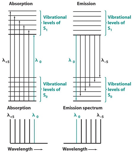
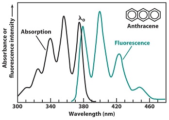
Fluorescence and phosphorescence come at lower energy than absorption (the excitation energy). As shown in Figure \(\PageIndex{1}\), in absorption, wavelength λ0 corresponds to a transition from the ground vibrational level of S0 to the lowest vibrational level of S1. After absorption, the vibrationally excited S1 molecule relaxes back to the lowest vibrational level of S1 prior to emitting any radiation. The highest energy transition comes at wavelength λ0, with a series of peaks following at longer wavelength. The absorption and emission spectra will have an approximate mirror image relation if the spacings between vibrational levels are roughly equal and if the transition probabilities are similar. The λ0 transitions in Figure \(\PageIndex{2}\), do not exactly overlap. As shown in Figure \(\PageIndex{8}\), a molecule absorbing radiation is initially in its electronic ground state, S0. This molecule possesses a certain geometry and solvation. As the electronic transition is faster than the vibrational motion of atoms or the translational motion of solvent molecules, when radiation is first absorbed, the excited S1 molecule still possesses its S0 geometry and solvation. Shortly after excitation, the geometry and solvation change to their most favorable values for S1 state. This rearrangement lowers the energy of excited molecule. When an S1 molecule fluoresces, it returns to the S0 state with S1 geometry and solvation. This unstable configuration must have a higher energy than that of an S0molecule with S0 geometry and solvation. The net effect in Figure \(\PageIndex{1}\) is that the λ0 emission energy is less than the λ0 excitation energy.
Instrumentation
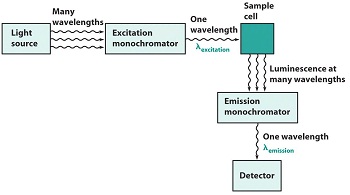
A schematic of an emiision experiment is give in Figure \(\PageIndex{3}\). An excitation wavelength is selected by one monochromator, and luminescence is observed through a second monochromator, usually positioned at 90° to the incident light to minimize the intensity of scattered light reaching the dector. If the excitation wavelength is fixed and the emitted radiation is scanned, an emission spectrum is produced.
Relationship to UV-vis Spectroscopy
Ultraviolet-visible (UV-vis) spectroscopy or ultraviolet-visible spectrophotometry refers to absorption spectroscopy or reflectance spectroscopy in the untraviolet-visible spectral region. The absorption or reflectance in the visible range directly affects the perceived color of the chemicals involved. In the UV-vis spectrum, an absorbance versus wavelength graph results and it measures transitions from the ground state to excited state, while photoluminescence deals with transitions from the excited state to the ground state.
An excitation spectrum is a graph of emission intensity versus excitation wavelength. An excitation spectrum looks very much like an absorption spectrum. The greater the absorbance is at the excitation wavelength, the more molecules are promoted to the excited state and the more emission will be observed.
By running an UV-vis absorption spectrum, the wavelength at which the molecule absorbs energy most and is excited to a large extent can be obtained. Using such value as the excitation wavelength can thus provide a more intense emission at a red-shifted wavelength, which is usually within twice of the excitation wavelength.
Applications
Detection of ACQ or AIE properties
Aggregation-caused quenching (ACQ) of light emission is a general phenomenon for many aromatic compounds that fluorescence is weakened with an increase in its solution concentration and even condensed phase. Such effect, however, comes into play in the solid state, which has prevented many lead luminogens identified by the laboratory solution-screening process from finding real-world applications in an engineering robust form.
Aggregation-induced emission (AIE), on the other hand, is a novel phenomenon that aggregation plays a constructive, instead of destructive role in the light-emitting process, which is exactly opposite to the ACQ effect.
A Case Study
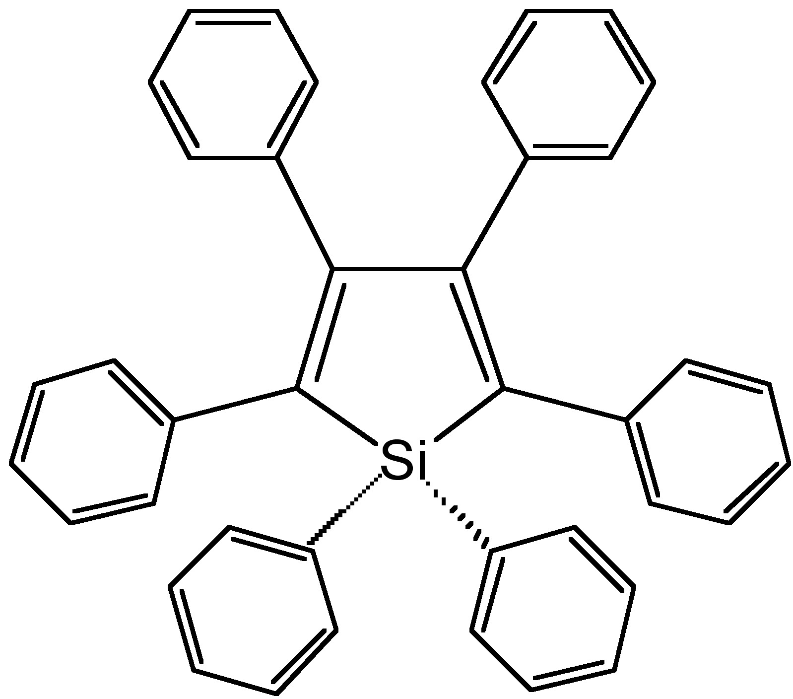
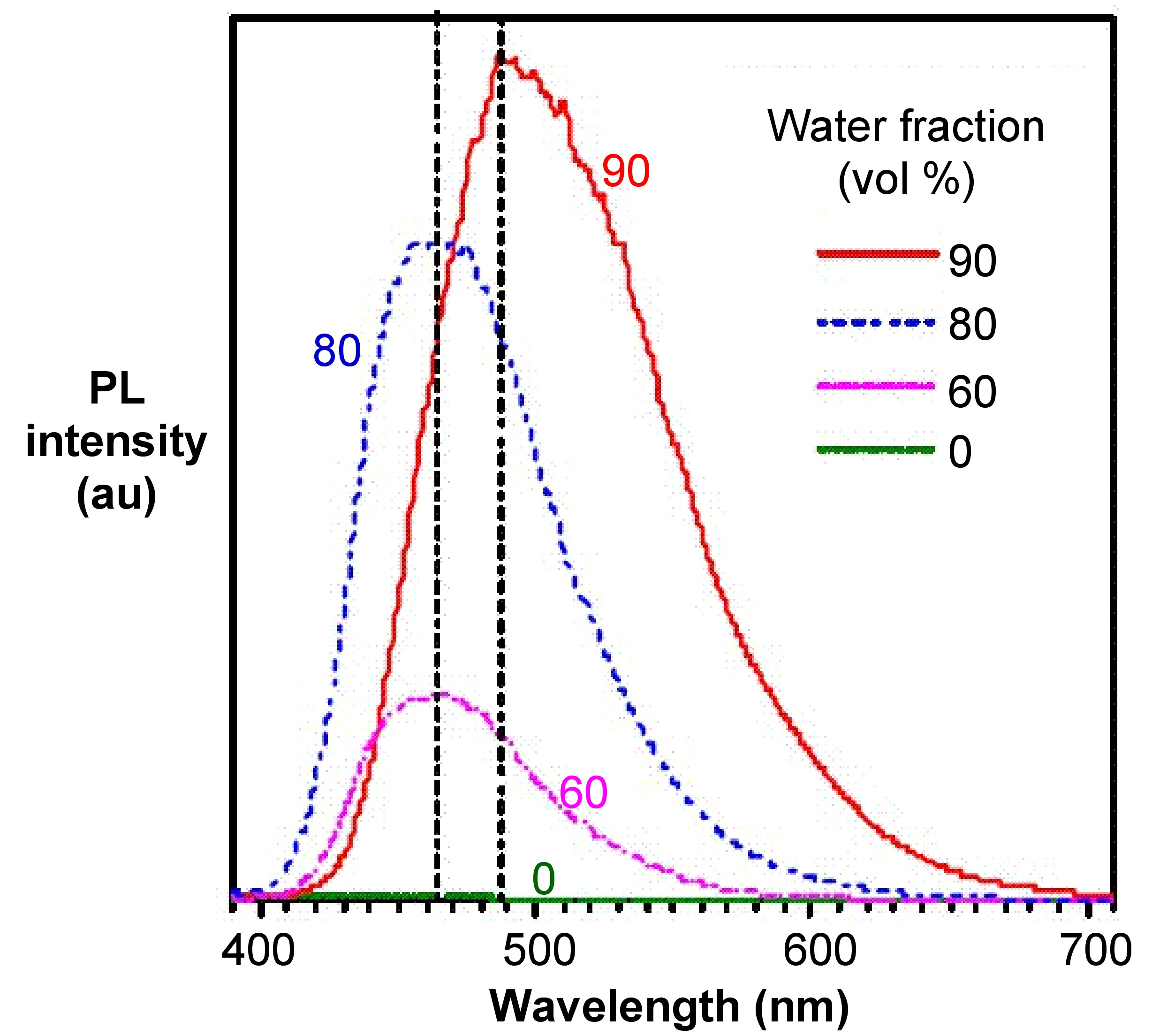
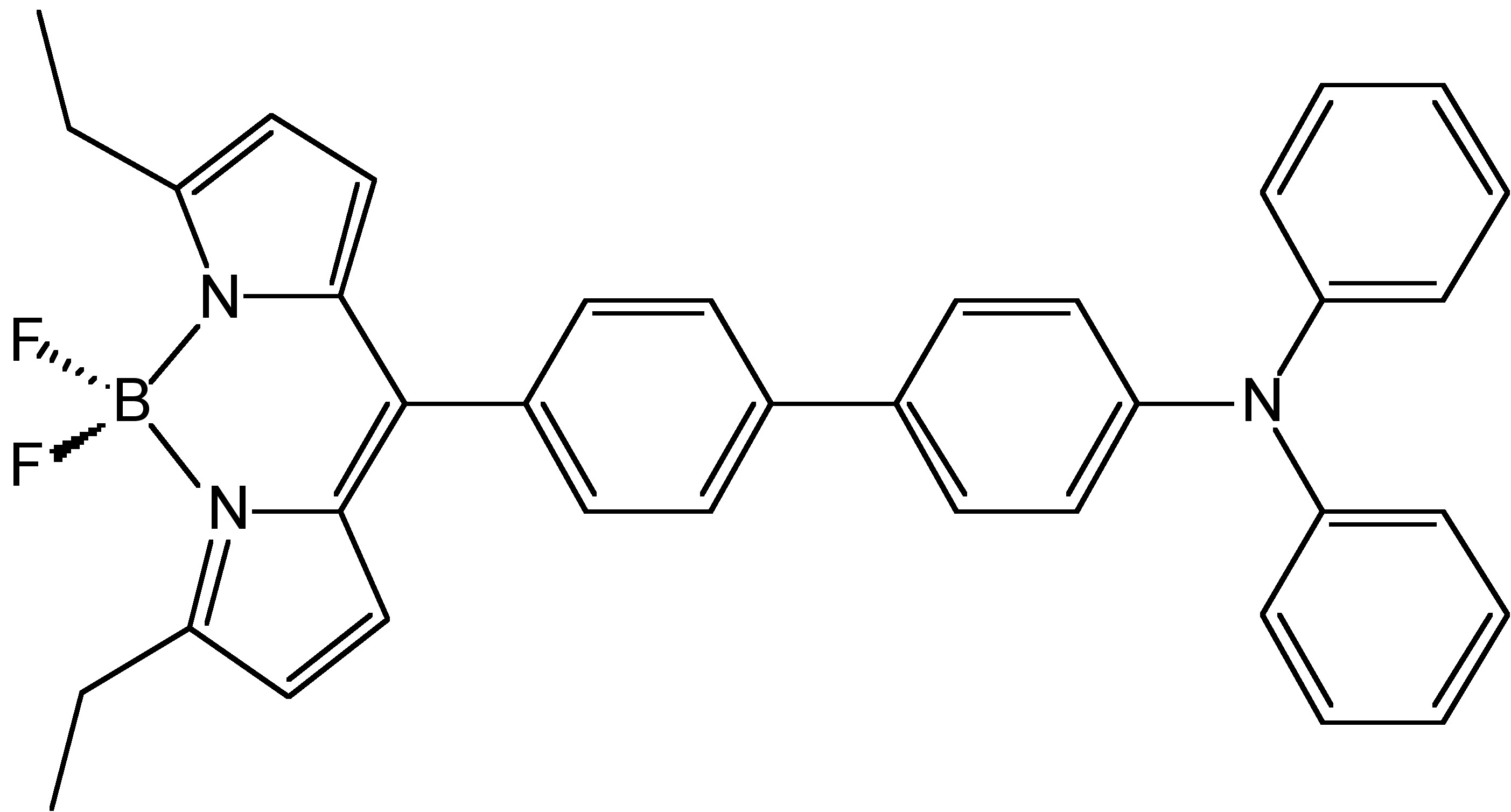
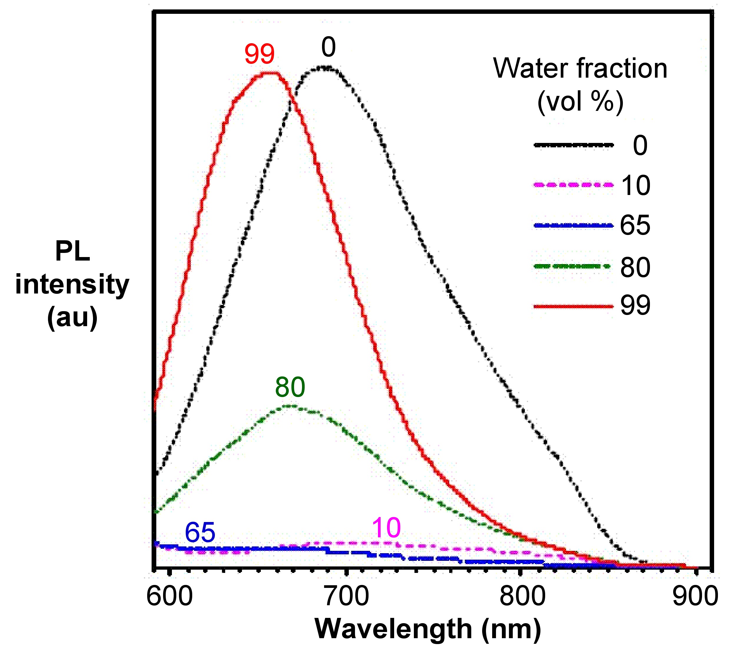
From the photoluminescence spectra of hexaphenylsilole (HPS, Figure \(\PageIndex{4}\)) show in Figure \(\PageIndex{5}\), it can be seen that as the water (bad solvent) fraction increases, the emission intensity of HPS increases. For BODIPY derivative Figure \(\PageIndex{6}\) in Figure \(\PageIndex{7}\), it shows that the PL intensity peaks at 0 water content resulted from intramolecular rotation or twisting, known as twisted intramolecular charge transfer (TICT).
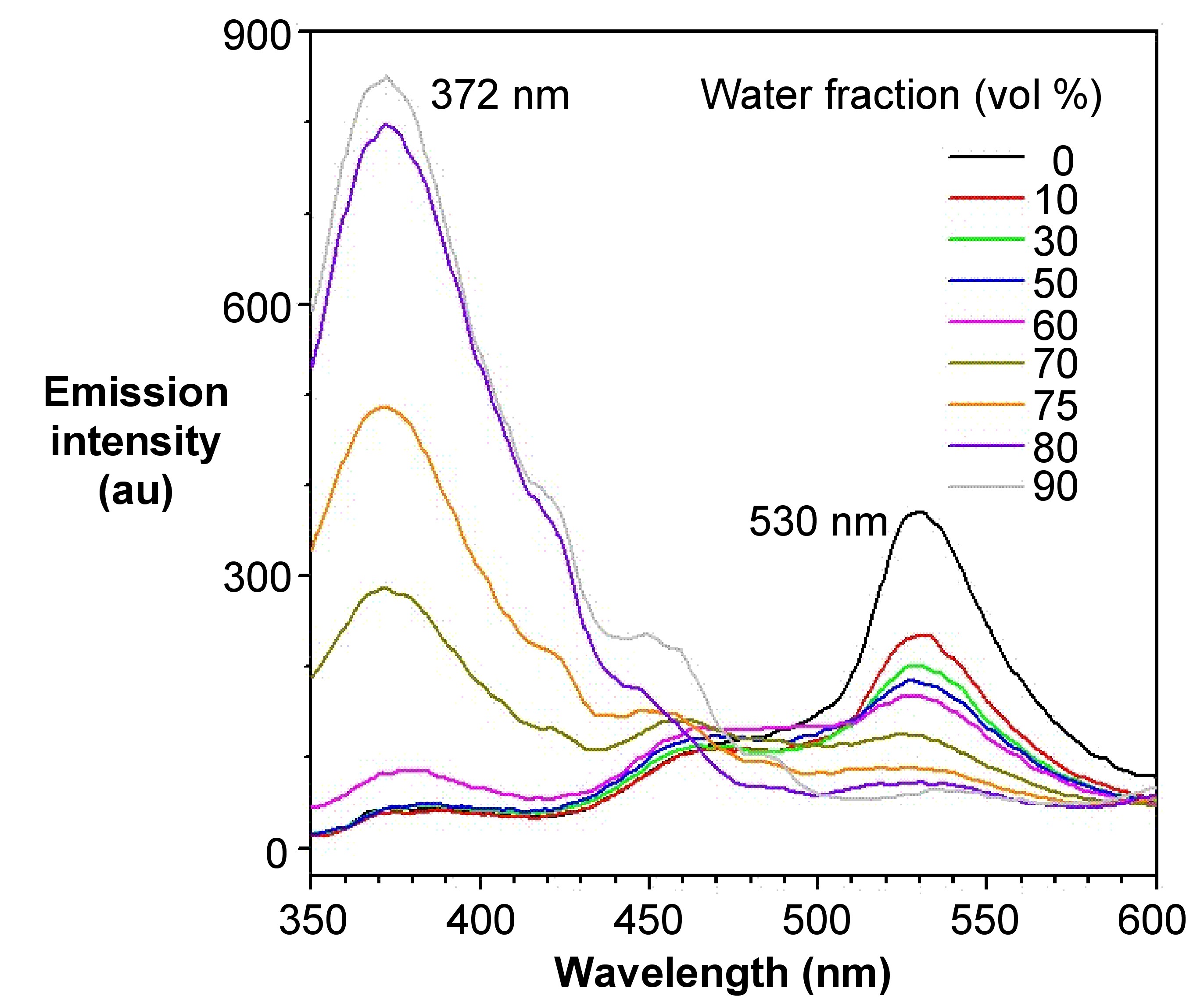
The emission color of an AIE luminogen is scarcely affected by solvent polarity, whereas that of a TICT luminogen typically bathochromically shifts with increasing solvent polarity. In Figure \(\PageIndex{8}\), however, it shows different patterns of emission under different excitation wavelengths. At the excitation wavelength of 372 nm, which is corresponding to the BODIPY group, the emission intensity increases as water fraction increases. However, it decreases at the excitation wavelength of 530 nm, which is corresponding to the TPE group. The presence of two emissions in this compound is due to the presence of two independent groups in the compound with AIE and ACQ properties, respectively.
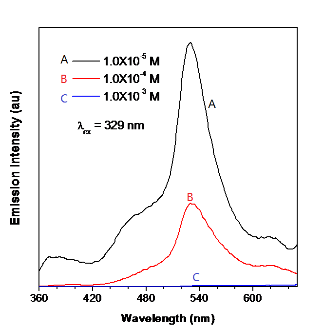
Detection of Luminescence with Respect to Molarity
Figure \(\PageIndex{9}\) shows the photoluminescence spectroscopy of a BODIPY-TPE derivative of different concentrations. At the excitation wavelength of 329 nm, as the molarity increases, the emission intensity decreases. Such compounds whose PL emission intensity enhances at low concentration can be a good chemo-sensor for the detection of the presence of compounds with low quantity.
Other Applications
Apart from the detection of light emission patterns, photoluminescence spectroscopy is of great significance in other fields of analysis, especially semiconductors.
Band Gap Determination
Band gap is the energy difference between states in the conduction and valence bands, of the radiative transition in semiconductors. The spectral distribution of PL from a semiconductor can be analyzed to nondestructively determine the electronic band gap. This provides a means to quantify the elemental composition of compound semiconductor and is a vitally important material parameter influencing solar cell device efficiency.
Impurity Levels and Defect Detection
Radiative transitions in semiconductors involve localized defect levels. The photoluminescence energy associated with these levels can be used to identify specific defects, and the amount of photoluminescence can be used to determine their concentration. The PL spectrum at low sample temperatures often reveals spectral peaks associated with impurities contained within the host material. Fourier transform photoluminescence microspectroscopy, which is of high sensitivity, provides the potential to identify extremely low concentrations of intentional and unintentional impurities that can strongly affect material quality and device performance.
Recombination Mechanisms
The return to equilibrium, known as “recombination”, can involve both radiative and nonradiative processes. The quantity of PL emitted from a material is directly related to the relative amount of radiative and nonradiative recombination rates. Nonradiative rates are typically associated with impurities and the amount of photoluminescence and its dependence on the level of photo-excitation and temperature are directly related to the dominant recombination process. Thus, analysis of photoluminescence can qualitatively monitor changes in material quality as a function of growth and processing conditions and help understand the underlying physics of the recombination mechanism.
Surface and Structure and Excited States
The widely used conventional methods such as XRD, IR and Raman spectroscopy, are very often not sensitive enough for supported oxide catalysts with low metal oxide concentrations. Photoluminescence, however, is very sensitive to surface effects or adsorbed species of semiconductor particles and thus can be used as a probe of electron-hole surface processes.
Limitations of Photoluminescence Spectroscopy
Very low concentrations of optical centers can be detected using photoluminescence, but it is not generally a quantitative technique. The main scientific limitation of photoluminescence is that many optical centers may have multiple excited states, which are not populated at low temperature.
The disappearance of luminescence signal is another limitation of photoluminescence spectroscopy. For example, in the characterization of photoluminescence centers of silicon no sharp-line photoluminescence from 969 meV centers was observed when they had captured self-interstitials.
Fluorescence Characterization and DNA Detection
Luminescence is a process involving the emission of light from any substance, and occurs from electronically excited states of that substance. Normally, luminescence is divided into two categories, fluorescence and phosphorescence, depending on the nature of the excited state.
Fluorescence is the emission of electromagnetic radiation light by a substance that has absorbed radiation of a different wavelength. Phosphorescence is a specific type of photoluminescence related to fluorescence. Unlike fluorescence, a phosphorescent material does not immediately re-emit the radiation it absorbs.
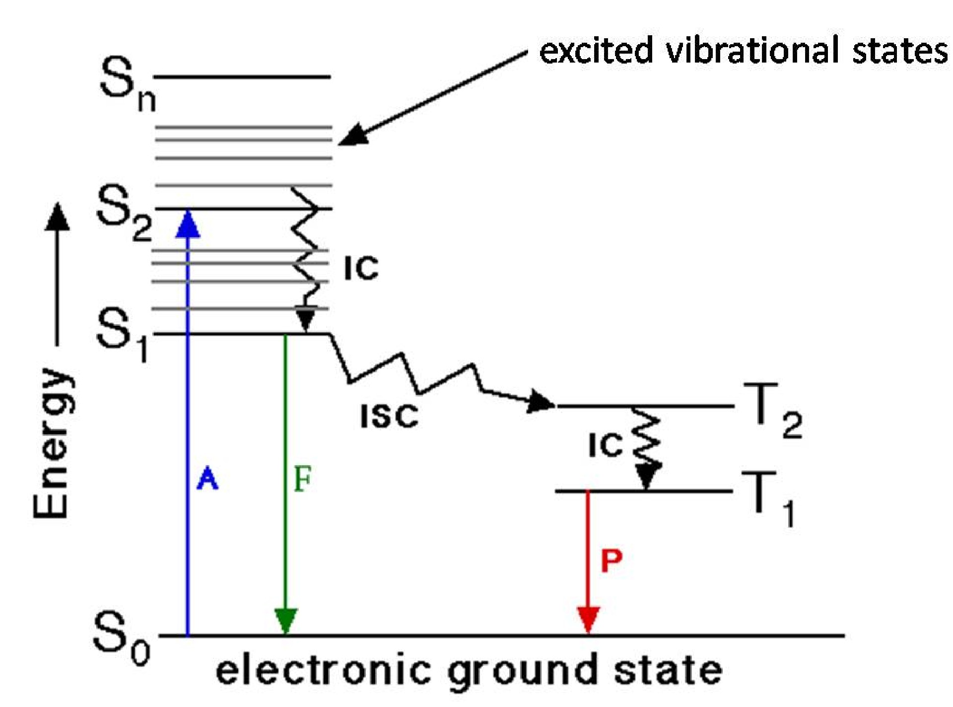
The process of fluorescent absorption and emission is easily illustrated by the Jablonski diagram. A classic Jablonski diagram is shown in Figure \(\PageIndex{10}\), where Sn represents the nth electronic states. There are different vibrational and rotational states in every electronic state. After light absorption, a fluorophore is excited to a higher electronic and vibrational state from ground state (here rotational states are not considered for simplicity). By internal conversion of energy, these excited molecules relax to lower vibrational states in S1 (Figure \(\PageIndex{10}\)) and then return to ground states by emitting fluorescence. Actually, excited molecules always return to higher vibration states in S0 and followed by some thermal process to ground states in S1. It is also possible for some molecules to undergo intersystem crossing process to T2 states (Figure \(\PageIndex{10}\)). After internal conversion and relaxing to T1, these molecules can emit phosphorescence and return to ground states.
The Stokes shift, the excited state lifetime and quantum yield are the three most important characteristics of fluorescence emission. Stokes shift is the difference between positions of the band maxima of the absorption and emission spectra of the same electronic transition. According to mechanism discussed above, an emission spectrum must have lower energy or longer wavelength than absorption light. The quantum yield is a measure of the intensity of fluorescence, as defined by the ratio of emitted photons over absorbed photons. Excited state lifetime is a measure of the decay times of the fluorescence.
Instrumentation of Fluorescence Spectroscopy
Spectrofluorometers
Most spectrofluorometers can record both excitation and emission spectra. An emission spectrum is the wavelength distribution of an emission measured at a single constant excitation wavelength. In comparison, an excitation spectrum is measured at a single emission wavelength by scanning the excitation wavelength.
Light Sources
Specific light sources are chosen depending on the application.
Arc and Incandescent Xenon Lamps
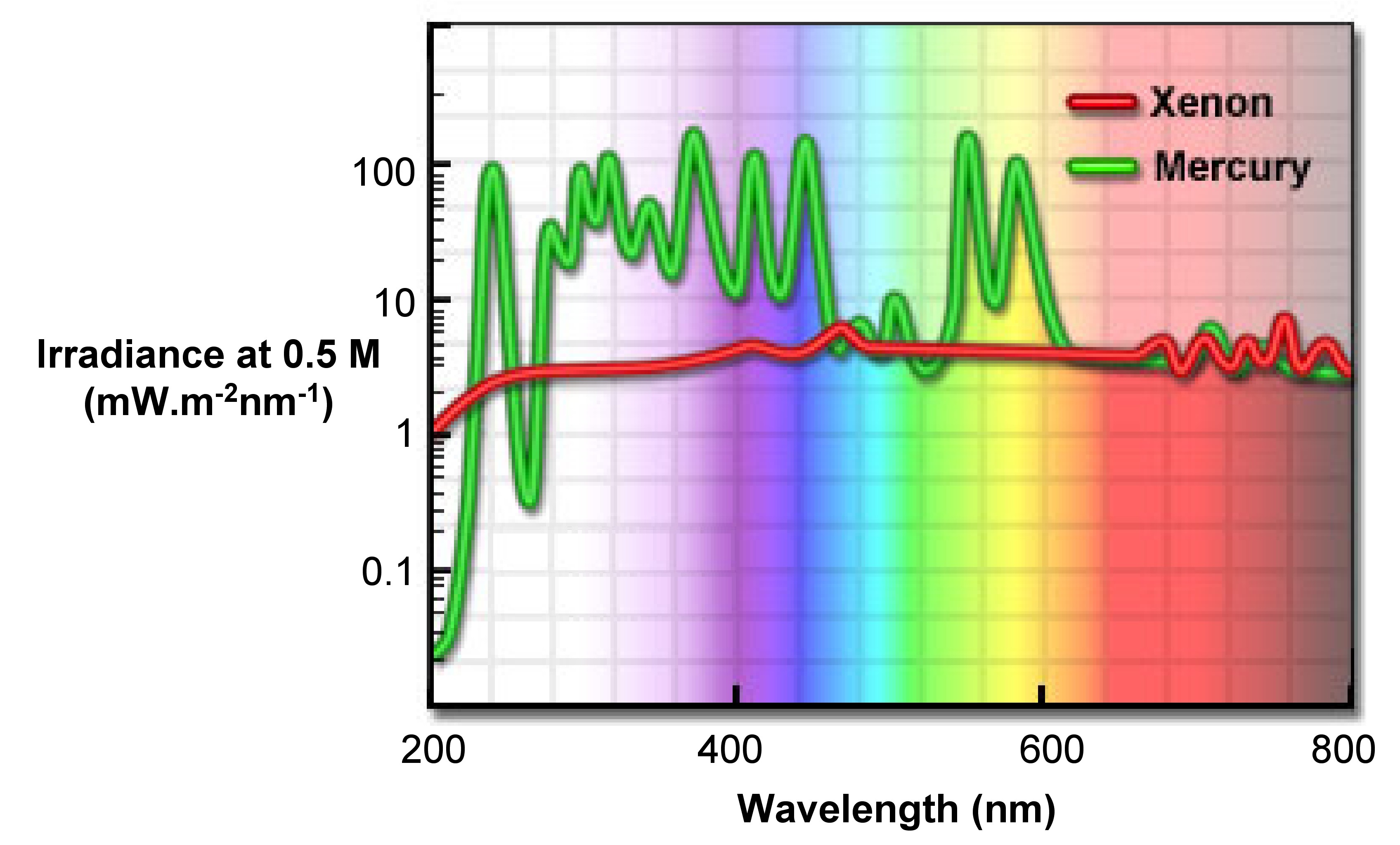
The high-pressure xenon (Xe) arc is the most versatile light source for steady-state fluorometers now. It can provides a steady light output from 250 - 700 nm (Figure \(\PageIndex{11}\)), with only some sharp lines near 450 and 800 nm. The reason that xenon arc lamps emit a continuous light is the recombination of electrons with ionized Xe atoms. These ions produced by collision between Xe and electrons. Those sharp lines near 450 nm are due to the excited Xe atoms that are not ionized.
During fluorescence experiment, some distortion of the excitation spectra can be observed, especially the absorbance locating in visible and ultraviolet region. Any distortion displayed in the peaks is the result of wavelength-dependent output of Xe lamps. Therefore, we need to apply some mathematic and physical approaches for correction.
High Pressure Mercury Lamps
Compared with xenon lamps, Hg lamps have higher intensities. As shown in Figure \(\PageIndex{11}\) the intensity of Hg lamps is concentrated in a series of lines, so it is a potentially better excitation light source if matched to certain fluorophorescence.
Xe-Hg Arc Lamps
High-pressure xenon-mercury lamps have been produced. They have much higher intensity in ultraviolet region than normal Xe lamps. Also, the introduction of Xe to Hg lamps broadens the sharp-line output of Hg lamps. Although the wavelength of output is still dominated by those Hg lines, these lines are broadened and fit to various fluorophores better. The Xe-Hg lamp output depends on the operating temperature.
Low Pressure Hg and Hg-Ar Lamps
Due to their very sharp line spectra, they are primarily useful for calibration purpose. The combination of Hg and Ar improve the output scale, from 200 - 1000 nm.
Other Light Source
There are many other light source for experimental and industrial application, such as pulsed xenon lamps, quartz-tungsten halogen (QTH) lamps, LED light sources, etc.
Monochromators
Most of the light sources used provide only polychromatic or white light. However, what is needed for experiments are various chromatic light with a wavelength range of 10 nm. Monocharomators help us to achieve this aim. Prisms and diffraction gratings are the two main kinds of monochromators used, although diffraction gratings are most useful, especially in spectrofluorometers.
Dispersion, efficiency, stray light level and resolution are important parameters for monochromators. Dispersion is mainly determined by slit width and expressed in nm/mm. It is prepared to have low stray light level. Stray light is defined as light transmitted by the monochromator at wavelength outside the chosen range. Also, a high efficiency is required to increase the ability to detect low light levels. Resolution depends on the slit width. There are normally two slits, entrance and exit in a fluorometers. Light intensity that passes through the slits is proportional to the square of the slit width. Larger slits have larger signal levels, but lower resolution, and vice verse. Therefore, it is important to balance the signal intensity and resolution with the slit width.
Optical filters
Optical filters are used in addition to monochromators, because the light passing through monochromator is rarely ideal, optical filters are needed for further purifying light source. If the basic excitation and emission properties of a particular system under study, then selectivity by using optical filters is better than by the use of monochromators. Two kinds of optical filter are gradually employed: colored filters and thin-film filters.
Colored Filters
Colored filters are the most traditional filter used before thin-film filter were developed. They can be divided into two categories: monochromatic filter and long-pass filter. The first one only pass a small range of light (about 10 - 25 nm) centered at particular chosen wavelength. In contrast, long pass filter transmit all wavelengths above a particular wavelength. In using these bandpass filters, special attention must be paid to the possibility of emission from the filter itself, because many filters are made up of luminescent materials that are easily excited by UV light. In order to avoid this problem, it is better to set up the filter further away from the sample.
Thin-film Filters
The transmission curves of colored class filter are not suitable for some application and as such they are gradually being substituted by thin-film filters. Almost any desired transmission curve can be obtained using a thin film filter.
Detectors
The standard detector used in many spectrofluorometers is the InGaAs array, which can provides rapid and robust spectral characterization in the near-IR. And the liquid-nitrogen cooling is applied to decrease the background noise. Normally, detectors are connected to a controller that can transfer a digital signal to and from the computer.
Fluorophores
At present a wide range of fluorophores have been developed as fluorescence probes in bio-system. They are widely used for clinical diagnosis, bio-tracking and labeling. The advance of fluorometers has been accompanied with developments in fluorophore chemistry. Thousands of fluorophores have been synthesized, but herein four categories of fluorophores will be discussed with regard their spectral properties and application.
Intrinsic or Natural Fluorophores
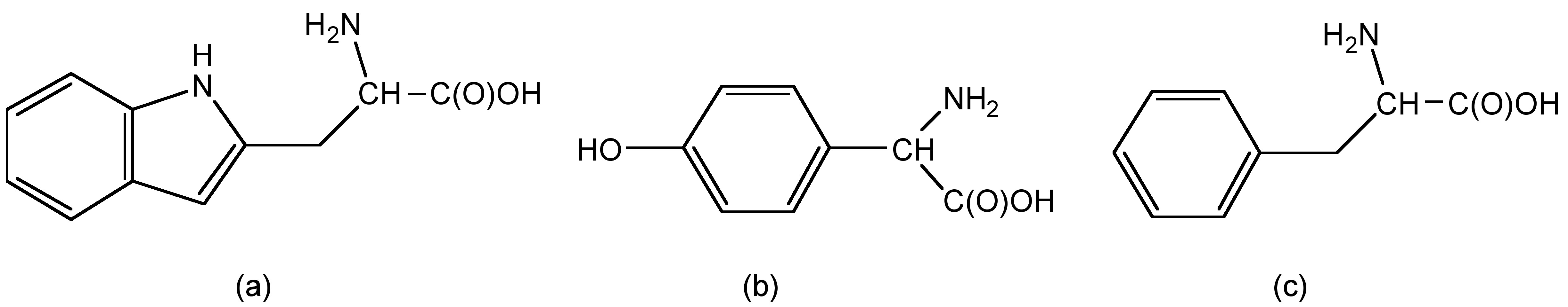
Tryptophan (trp), tyrosine (tyr), and phenylalanine (phe) are three natural amino acid with strong fluorescence (Figure \(\PageIndex{12}\)). In tryptophan, the indole groups absorbs excitation light as UV region and emit fluorescence.
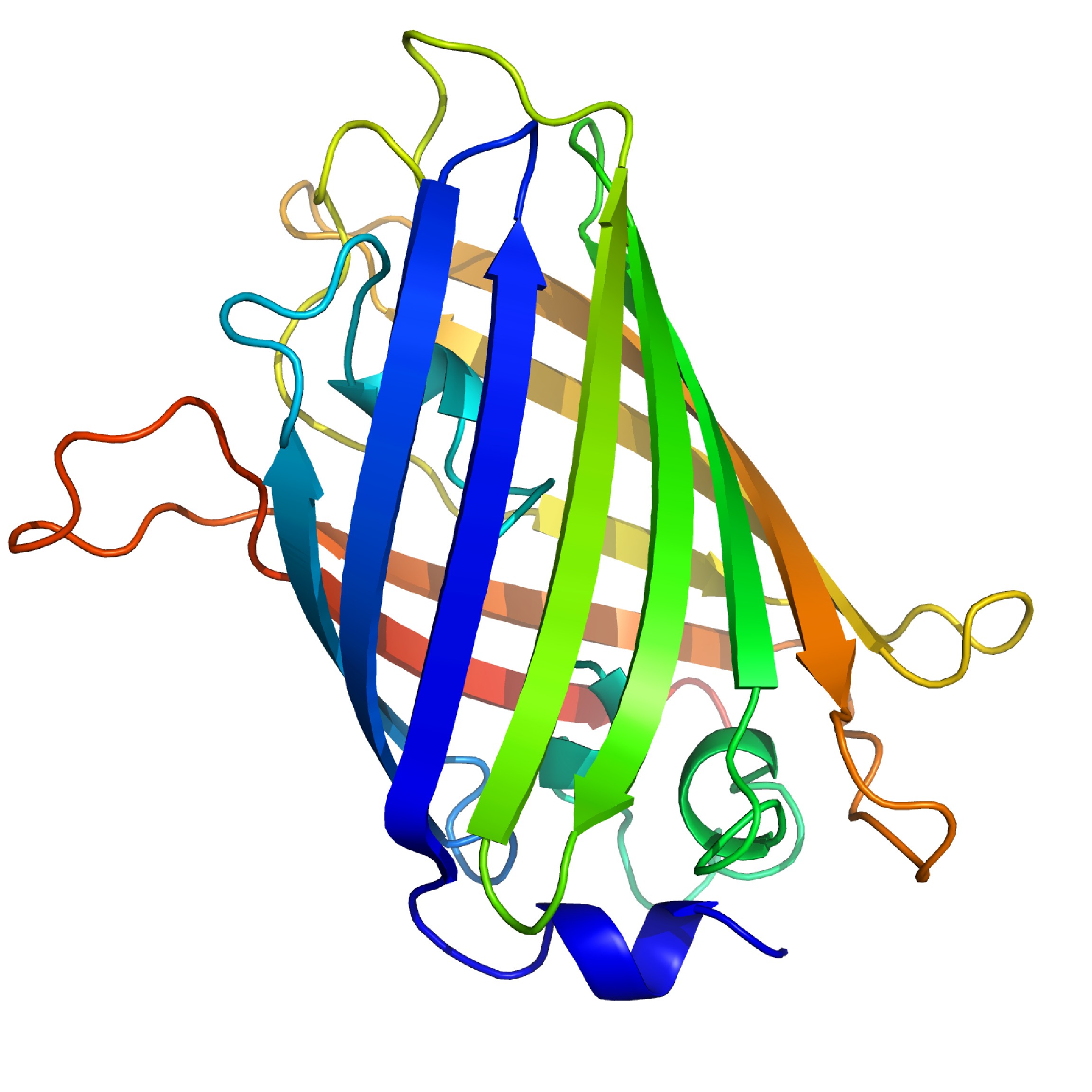
Green fluorescent proteins (GFP) is another natural fluorophores. GFP is composed of 238 amino acids (Figure \(\PageIndex{13}\)), and it exhibits a characteristic bright green fluorescence when excited. They are mainly extracted from bioluminescent jellyfish Aequorea vicroria, and are employed as signal reporters in molecular biology.
Extrinsic Fluorophores
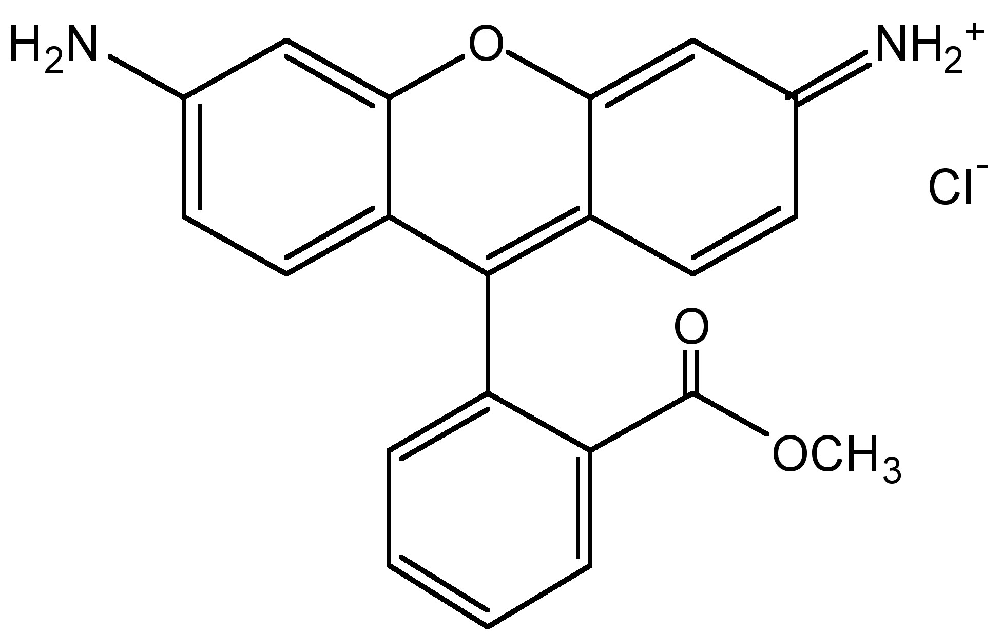
Most bio-molecules are nonfluorescent, therefore it is necessary to connect different fluorophores to enable labeling or tracking of the biomolecules. For example, DNA is an example of a biomolecule without fluorescence. The Rhodamine (Figure \(\PageIndex{14}\)) and BODIPY (Figure \(\PageIndex{15}\)) families are two kinds of well-developed organic fluorophores. They have been extensively employed in design of molecular probes due to their excellent photophysical properties.

Red and Near-infrared (NIR) dyes
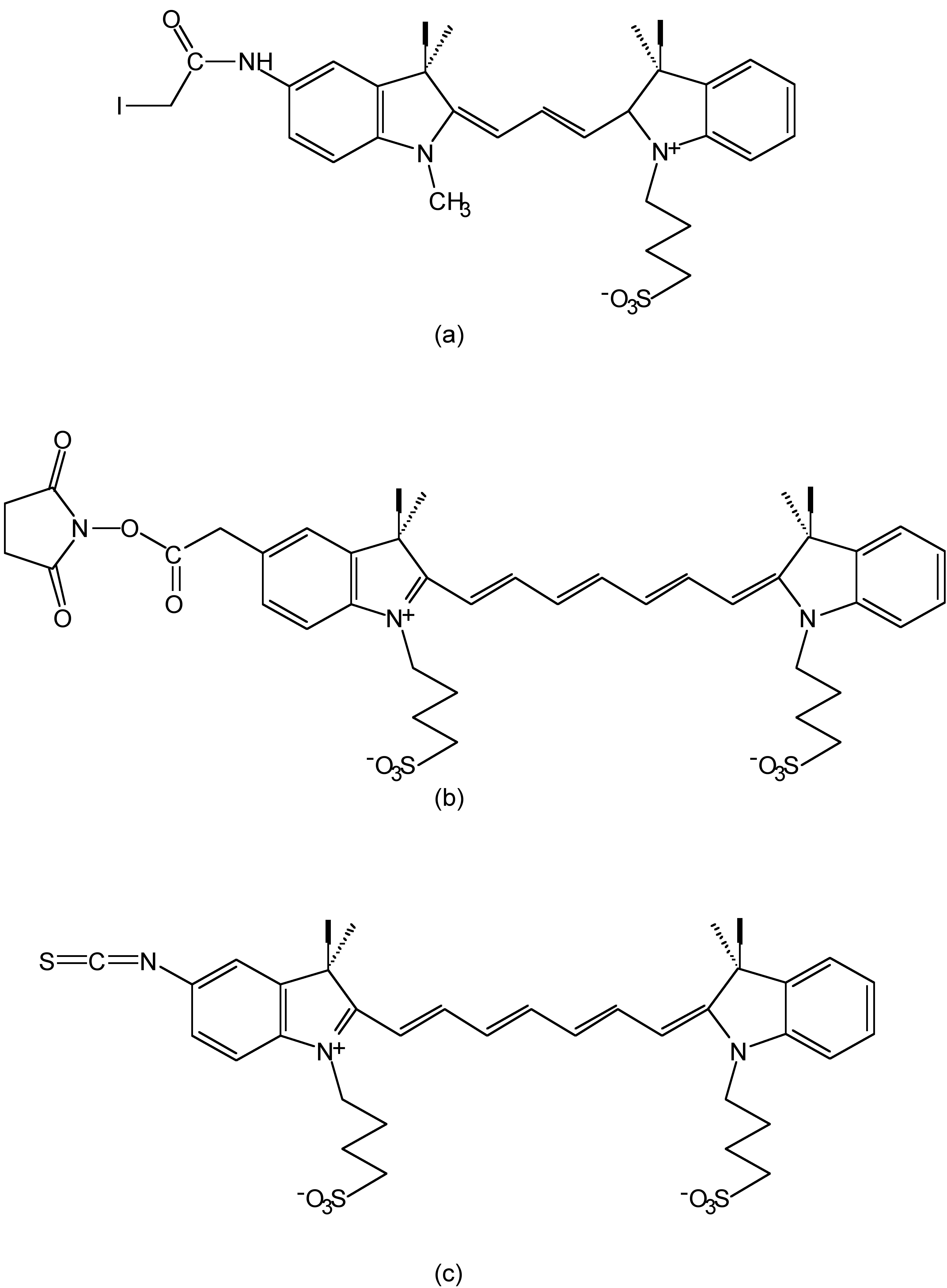
With the development of fluorophores, red and near-infrared (NIR) dyes attract increasing attention since they can improve the sensitivity of fluorescence detection. In biological system, autofluorescence always increase the ratio of signal-to-noise (S/N) and limit the sensitivity. As the excitation wavelength turns to longer, autopfluorescence decreases accordingly, and therefore signal-to-noise ratio increases. Cyanines are one such group of long-wavelength dyes, e.g., Cy-3, Cy-5 and Cy-7 (Figure \(\PageIndex{16}\)), which have emission at 555, 655 and 755 nm respectively.
Long-lifetime Fluorophores
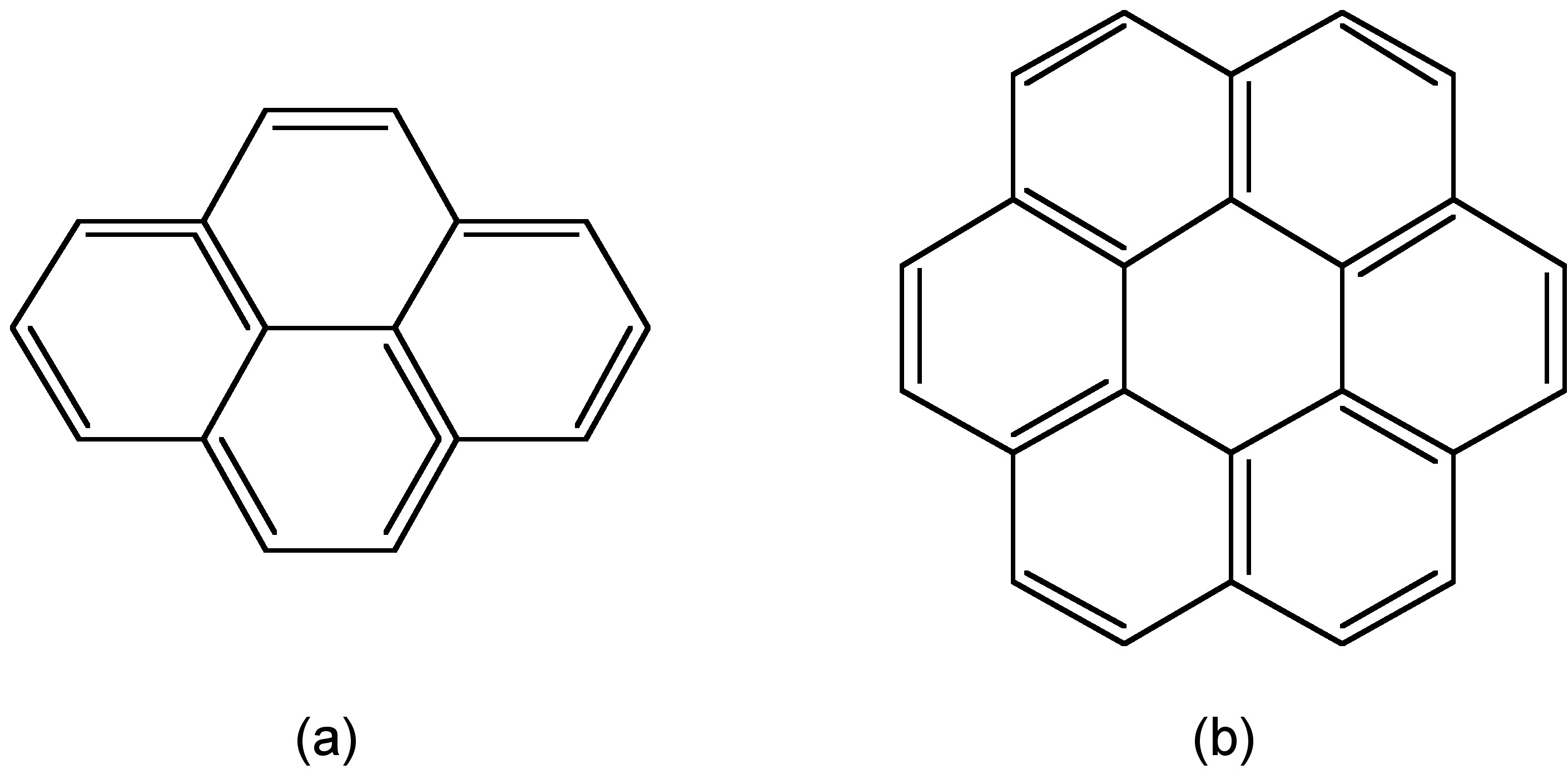
Almost all of the fluorophores mentioned above are organic fluorophores that have relative short lifetime from 1-10 ns. However, there are also a few long-lifetime organic fluorophore, such as pyrene and coronene with lifetime near 400 ns and 200 ns respectively (Figure \(\PageIndex{17}\)). Long-lifetime is one of the important properties to fluorophores. With its help, the autofluorescence in biological system can be removed adequately, and hence improve the detectability over background.
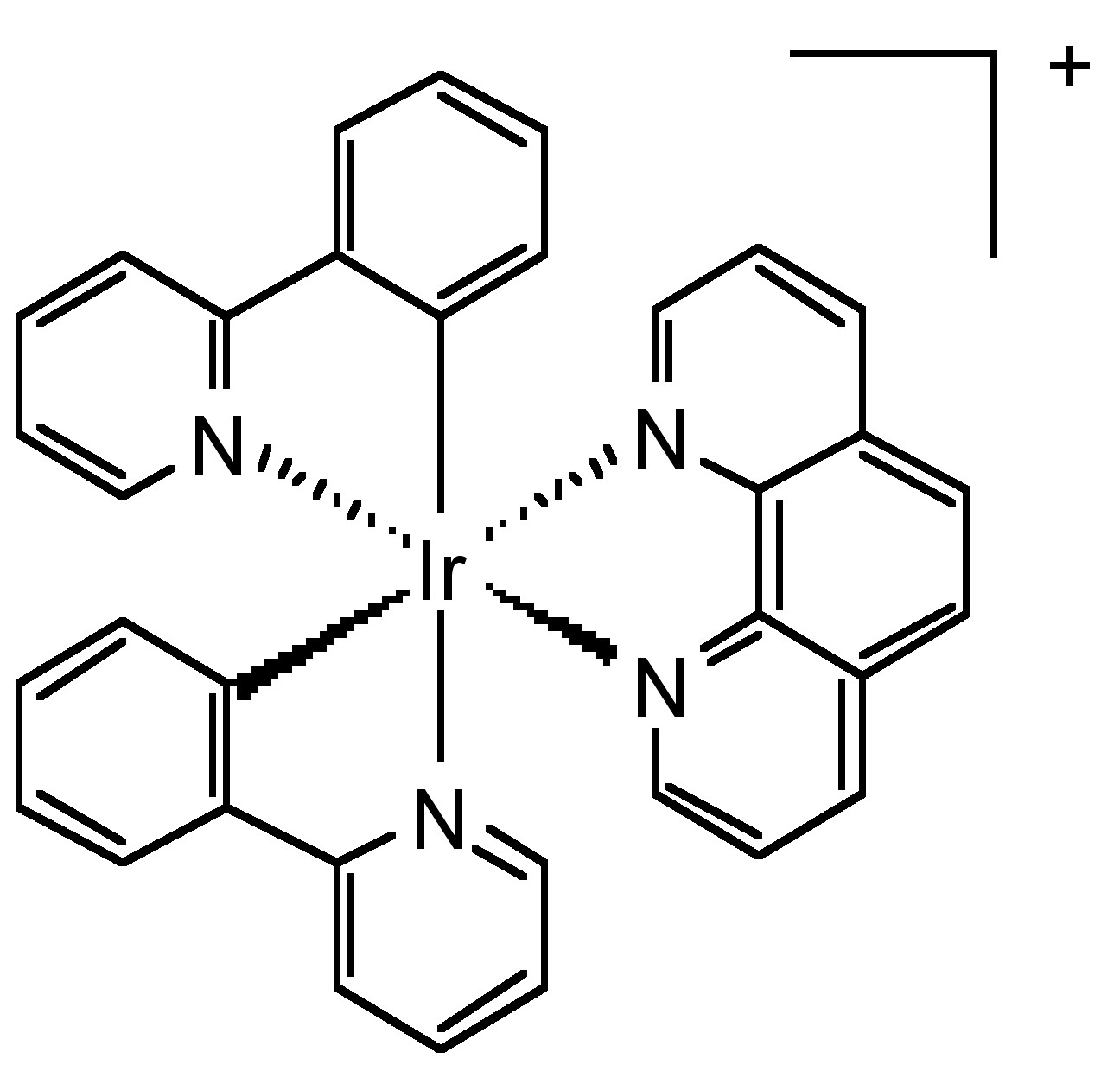
Although their emission belongs to phosphorescence, transition metal complexes are a significant class of long-lifetime fluorophores. Ruthenium (II), iridium (III), rhenium (I), and osmium (II) are the most popular transition metals that can combine with one to three diimine ligands to form fluorescent metal complexes. For example, iridium forms a cationic complex with two phenyl pyridine and one diimine ligand (Figure \(\PageIndex{18}\)). This complex has excellent quantum yield and relatively long lifetime.
Applications
With advances in fluorometers and fluorophores, fluorescence has been a dominant techonology in the medical field, such clinic diagnosis and flow cytometry. Herein, the application of fluorescence in DNA and RNA detecition is discussed.
The low concentration of DNA and RNA sequences in cells determine that high sensitivity of the probe is required, while the existence of various DNA and RNA with similar structures requires a high selectivity. Hence, fluorophores were introduced as the signal group into probes, because fluorescence spectroscopy is most sensitive technology until now.
The general design of a DNA or RNA probe involves using an antisense hybridization oligonucleotide to monitor target DNA sequence. When the oligonucleotide is connected with the target DNA, the signal groups-the fluorophores-emit designed fluorescence. Based on fluorescence spectroscopy, signal fluorescence can be detected which help us to locate the target DNA sequence. The selectively inherent in the hybridization between two complementary DNA/RNA sequences make this kind of DNA probes extremely high selectivity. A molecular Beacon is one kind of DNA probes. This simple but novel design is reported by Tyagi and Kramer in 1996 (Figure \(\PageIndex{19}\)) and gradually developed to be one of the most common DNA/RNA probes.
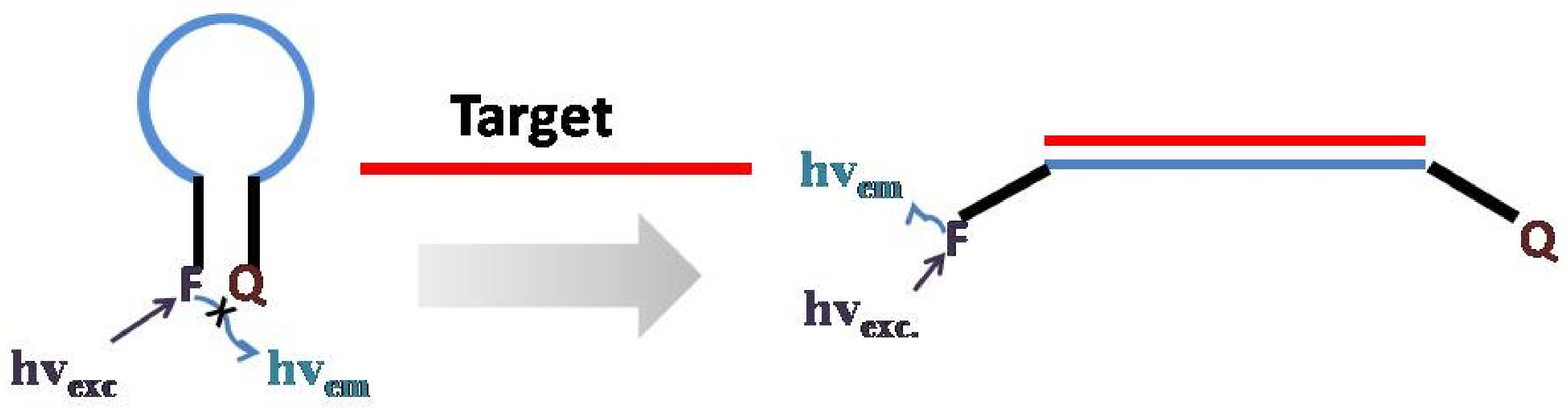
Generally speaking, a molecular beacon it is composed of three parts: one oligonucleotide, a fluorophore and a quencher at different ends. In the absence of the target DNA, the molecular beacon is folded like a hairpin due to the interaction between the two series nucleotides at opposite ends of the oligonucleotide. At this time, the fluorescence is quenched by the close quencher. However, in the presence of the target, the probe region of the MB will hybridize to the target DNA, open the folded MB and separate the fluorophore and quencher. Therefore, the fluorescent signal can be detected which indicate the existence of a particular DNA.
Fluorescence Correlation Spectroscopy
Florescence correlation spectroscopy (FCS) is an experimental technique that that measures fluctuations in fluorescence intensity caused by the Brownian motion of particles. Fluorescence is a form of luminescence that involves the emission of light by a substance that has absorbed light or other electromagnetic radiation. Brownian motion is the random motion of particles suspended in a fluid that results from collisions with other molecules or atoms in the fluid. The initial experimental data is presented as intensity over time but statistical analysis of fluctuations makes it possible to determine various physical and photo-physical properties of molecules and systems. When combined with analysis models, FCS can be used to find diffusion coefficients, hydrodynamic radii, average concentrations, kinetic chemical reaction rates, and single-triplet state dynamics. Singlet and triplet states are related to electron spin. Electrons can have a spin of (+1/2) or (-1/2). For a system that exists in the singlet state, all spins are paired and the total spin for the system is ((-1/2) + (1/2)) or 0. When a system is in the triplet state, there exist two unpaired electrons with a total spin state of 1.
History
The first scientists to be credited with the application of fluorescence to signal-correlation techniques were Douglas Magde, Elliot L. Elson, and Walt W.Webb, therefore they are commonly referred to as the inventors of FCS. The technique was originally used to measure the diffusion and binding of ethidium bromide (Figure \(\PageIndex{20}\)) onto double stranded DNA.

Initially, the technique required high concentrations of fluorescent molecules and was very insensitive. Starting in 1993, large improvements in technology and the development of confocal microscopy and two-photon microscopy were made, allowing for great improvements in the signal to noise ratio and the ability to do single molecule detection. Recently, the applications of FCS have been extended to include the use of FörsterResonance Energy Transfer (FRET), the cross-correlation between two fluorescent channels instead of auto correlation, and the use of laser scanning. Today, FCS is mostly used for biology and biophysics.
Instrumentation
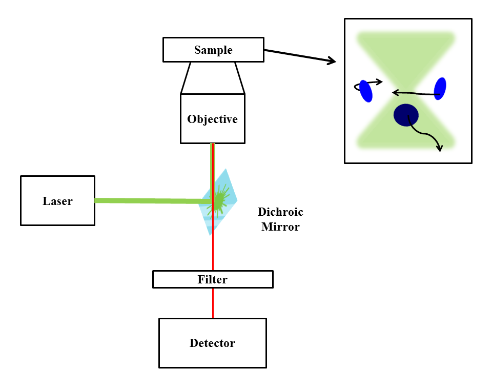
A basic FCS setup (Figure \(\PageIndex{21}\)) consists of a laser line that is reflected into a microscope objective by a dichroic mirror. The laser beam is focused on a sample that contains very dilute amounts of fluorescent particles so that only a few particles pass through the observed space at any given time. When particles cross the focal volume (the observed space) they fluoresce. This light is collected by the objective and passes through the dichroic mirror (collected light is red-shifted relative to excitation light), reaching the detector. It is essential to use a detector with high quantum efficiency (percentage of photons hitting the detector that produce charge carriers). Common types of detectors are a photo-multiplier tube (rarely used due to low quantum yield), an avalanche photodiode, and a super conducting nanowire single photo detector. The detector produces an electronic signal that can be stored as intensity over time or can be immediately auto correlated. It is common to use two detectors and cross- correlate their outputs leading to a cross-correlation function that is similar to the auto correlation function but is free from after-pulsing (when a photon emits two electronic pulses). As mentioned earlier, when combined with analysis models, FCS data can be used to find diffusion coefficients, hydrodynamic radii, average concentrations, kinetic chemical reaction rates, and single-triplet dynamics.
Analysis
When particles pass through the observed volume and fluoresce, they can be described mathematically as point spread functions, with the point of the source of the light being the center of the particle. A point spread function (PSF) is commonly described as an ellipsoid with measurements in the hundreds of nanometer range (although not always the case depending on the particle). With respect to confocal microscopy, the PSF is approximated well by a Gaussian, \ref{1}, where I0 is the peak intensity, r and z are radial and axial position, and wxy and wzare the radial and axial radii (with wz > wxy).
\[ PSF(r,z) \ =\ I_{0} e^{-2r^{2}}/\omega^{2}_{xy}e^{-2z^{2}/\omega^{2}_{z}} \label{1} \]
This Gaussian is assumed with the auto-correlation with changes being applied to the equation when necessary (like the case of a triplet state, chemical relaxation, etc.). For a Gaussian PSF, the autocorrelation function is given by \ref{2}, where \ref{3} is the stochastic displacement in space of a fluorophore after time T.
\[ G(\tau )\ =\frac{1}{\langle N \rangle } \langle exp (- \frac{\Delta (\tau)^{2} \ +\ \Delta Y(\tau )^{2}}{w^{2}_{xy}}\ -\ \frac{\Delta Z(\tau )^{2}}{w^{2}_{z}}) \rangle \label{2} \]
\[ \Delta \vec{R} (\tau )\ =\ (\Delta X(\tau ), \Delta (\tau ), \Delta (\tau )) \label{3} \]
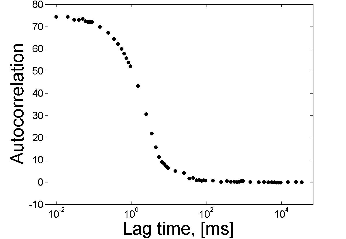
The expression is valid if the average number of particles, N, is low and if dark states can be ignored. Because of this, FCS observes a small number of molecules (nanomolar and picomolar concentrations), in a small volume (~1μm3) and does not require physical separation processes, as information is determined using optics. After applying the chosen autocorrelation function, it becomes much easier to analyze the data and extract the desired information (Figure \(\PageIndex{22}\)).
Application
FCS is often seen in the context of microscopy, being used in confocal microscopy and two-photon excitation microscopy. In both techniques, light is focused on a sample and fluorescence intensity fluctuations are measured and analyzed using temporal autocorrelation. The magnitude of the intensity of the fluorescence and the amount of fluctuation is related to the number of individual particles; there is an optimum measurement time when the particles are entering or exiting the observation volume. When too many particles occupy the observed space, the overall fluctuations are small relative to the total signal and are difficult to resolve. On the other hand, if the time between molecules passing through the observed space is too long, running an experiment could take an unreasonable amount of time. One of the applications of FCS is that it can be used to analyze the concentration of fluorescent molecules in solution. Here, FCS is used to analyze a very small space containing a small number of molecules and the motion of the fluorescence particles is observed. The fluorescence intensity fluctuates based on the number of particles present; therefore analysis can give the average number of particles present, the average diffusion time, concentration, and particle size. This is useful because it can be done in vivo, allowing for the practical study of various parts of the cell. FCS is also a common technique in photo-physics, as it can be used to study triplet state formation and photo-bleaching. State formation refers to the transition between a singlet and a triplet state while photo-bleaching is when a fluorophore is photo-chemically altered such that it permanently looses its ability to fluoresce. By far, the most popular application of FCS is its use in studying molecular binding and unbinding often, it is not a particular molecule that is of interest but, rather, the interaction of that molecule in a system. By dye labeling a particular molecule in a system, FCS can be used to determine the kinetics of binding and unbinding (particularly useful in the study of assays).
Main Advantages and Limitations
| Advantage | Limitation |
|---|---|
| Can be used in vivo | Can be noisy depending on the system |
| Very sensitive | Does not work if concentration of dye is too high |
| The same instrumentation can perform various kinds of experiments | Raw data does not say much, analysis models must be applied |
| Has been used in various studies, extensive work has been done to establish the technique | If system deviates substantially from the ideal, analysis models can be difficult to apply (making corrections hard to calculate). |
| A large amount of information can be extracted | It may require more calculations to approximate PSF, depending on the particular shape. |
Molecular Phosphorescence Spectroscopy
When a material that has been radiated emits light, it can do so either via incandescence, in which all atoms in the material emit light, or via luminescence, in which only certain atoms emit light, Figure \(\PageIndex{23}\). There are two types of luminescence: fluorescence and phosphorescence. Phosphorescence occurs when excited electrons of a different multiplicity from those in their ground state return to their ground state via emission of a photon, Figure \(\PageIndex{24}\). It is a longer-lasting and less common type of luminescence, as it is a spin forbidden process, but it finds applications across numerous different fields. This module will cover the physical basis of phosphorescence, as well as instrumentation, sample preparation, limitations, and practical applications relating to molecular phosphorescence spectroscopy.
Phosphorescence
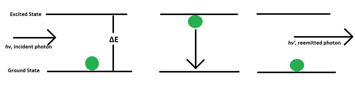
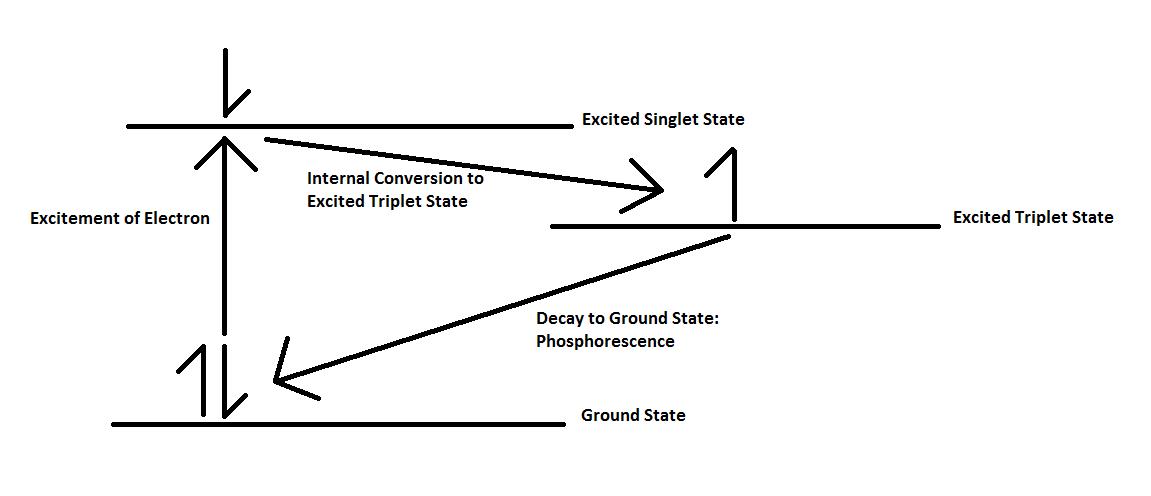
Phosphorescence is the emission of energy in the form of a photon after an electron has been excited due to radiation. In order to understand the cause of this emission, it is first important to consider the molecular electronic state of the sample. In the singlet molecular electronic state, all electron spins are paired, meaning that their spins are antiparallel to one another. When one paired electron is excited to a higher-energy state, it can either occupy an excited singlet state or an excited triplet state. In an excited singlet state, the excited electron remains paired with the electron in the ground state. In the excited triplet state, however, the electron becomes unpaired with the electron in ground state and adopts a parallel spin. When this spin conversion happens, the electron in the excited triplet state is said to be of a different multiplicity from the electron in the ground state. Phosphorescence occurs when electrons from the excited triplet state return to the ground singlet state, \ref{4} - \ref{6}, where E represents an electron in the singlet ground state, E* represent the electron in the singlet excited state, and T* represents the electron in the triplet excited state.
\[ E\ +\ hv \rightarrow E* \label{4} \]
\[ E* \rightarrow T* \label{5} \]
\[T* \rightarrow \ E\ +\ hv' \label{6} \]
Electrons in the triplet excited state are spin-prohibited from returning to the singlet state because they are parallel to those in the ground state. In order to return to the ground state, they must undergo a spin conversion, which is not very probable, especially considering that there are many other means of releasing excess energy. Because of the need for an internal spin conversion, phosphorescence lifetimes are much longer than those of other kinds of luminescence, lasting from 10-4 to 104 seconds.
Historically, phosphorescence and fluorescence were distinguished by the amount of time after the radiation source was removed that luminescence remained. Fluorescence was defined as short-lived chemiluminescence (< 10-5 s) because of the ease of transition between the excited and ground singlet states, whereas phosphorescence was defined as longer-lived chemiluminescence. However, basing the difference between the two forms of luminescence purely on time proved to be a very unreliable metric. Fluorescence is now defined as occurring when decaying electrons have the same multiplicity as those of their ground state.
Sample Preparation
Because phosphorescence is unlikely and produces relatively weak emissions, samples using molecular phosphorescence spectroscopy must be very carefully prepared in order to maximize the observed phosphorescence. The most common method of phosphorescence sample preparation is to dissolve the sample in a solvent that will form a clear and colorless solid when cooled to 77 K, the temperature of liquid nitrogen. Cryogenic conditions are usually used because, at low temperatures, there is little background interference from processes other than phosphorescence that contribute to loss of absorbed energy. Additionally, there is little interference from the solvent itself under cryogenic conditions. The solvent choice is especially important; in order to form a clear, colorless solid, the solvent must be of ultra-high purity. The polarity of the phosphorescent sample motivates the solvent choice. Common solvents include ethanol for polar samples and EPA (a mixture of diethyl ether, isopentane, and ethanol in a 5:5:2 ratio) for non-polar samples. Once a disk has been formed from the sample and solvent, it can be analyzed using a phosphoroscope.
Room Temperature Phosphorescence
While using a rigid medium is still the predominant choice for measuring phosphorescence, there have been recent advances in room temperature spectroscopy, which allows samples to be measured at warmer temperatures. Similar the sample preparation using a rigid medium for detection, the most important aspect is to maximize recorded phosphorescence by avoiding other forms of emission. Current methods for allowing good room detection of phosphorescence include absorbing the sample onto an external support and putting the sample into a molecular enclosure, both of which will protect the triplet state involved in phosphorescence.
Instrumentation and Measurement
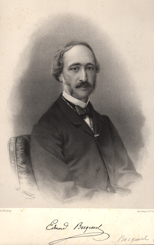
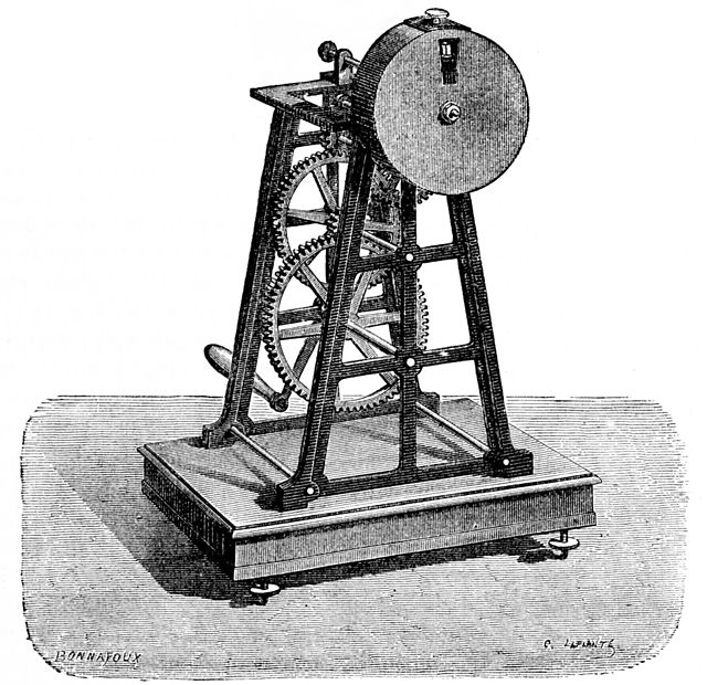
Phosphorescence is recorded in two distinct methods, with the distinguishing feature between the two methods being whether or not the light source is steady or pulsed. When the light source is steady, a phosphoroscope, or an attachment to a fluorescence spectrometer, is used. The phosphoroscope was experimentally devised by Alexandre-Edmond Becquerel, a pioneer in the field of luminescence, in 1857, Figure \(\PageIndex{25}\).
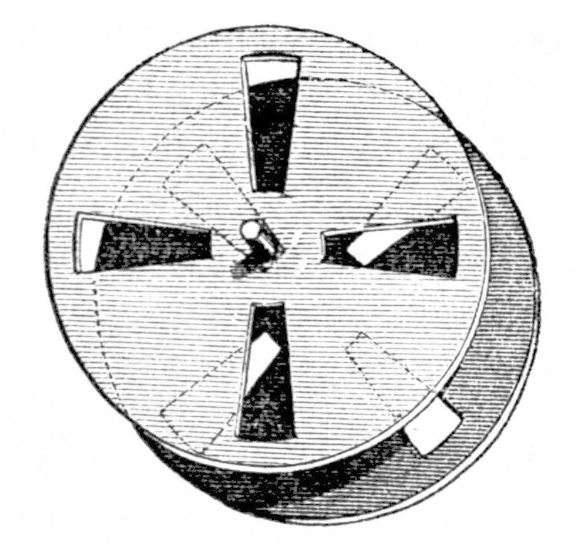
There are two different kinds of phosphoroscopes: rotating disk phosphoroscopes and rotating can phosphoroscopes. A rotating disk phosphoroscope, Figure \(\PageIndex{26}\), comprises two rotating disk with holes, in the middle of which is placed the sample to be tested. After a light beam penetrates one of the disks, the sample is electronically excited by the light energy and can phosphoresce; a photomultiplier records the intensity of the phosphorescence. Changing the speed of the disks’ rotation allows a decay curve to be created, which tells the user how long phosphorescence lasts.
The second type of phosphoroscope, the rotating can phosphoroscope, employs a rotating cylinder with a window to allow passage of light, Figure \(\PageIndex{27}\). The sample is placed on the outside edge of the can and, when light from the source is allowed to pass through the window, the sample is electronically excited and phosphoresces, and the intensity is again detected via photomultiplier. One major advantage of the rotating can phosphoroscope over the rotating disk phosphoroscope is that, at high speeds, it can minimize other types of interferences such as fluorescence and Raman and Rayleigh scattering, the inelastic and elastic scattering of photons, respectively.
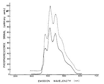
The more modern, advanced measurement of phosphorescence uses pulsed-source time resolved spectrometry and can be measured on a luminescence spectrometer. A luminescence spectrometer has modes for both fluorescence and phosphorescence, and the spectrometer can measure the intensity of the wavelength with respect to either the wavelength of the emitted light or time, Figure \(\PageIndex{28}\).
The spectrometer employs a gated photomultiplier to measure the intensity of the phosphorescence. After the initial burst of radiation from the light source, the gate blocks further light, and the photomultiplier measures both the peak intensity of phosphorescence as well as the decay, as shown in Figure \(\PageIndex{29}\).
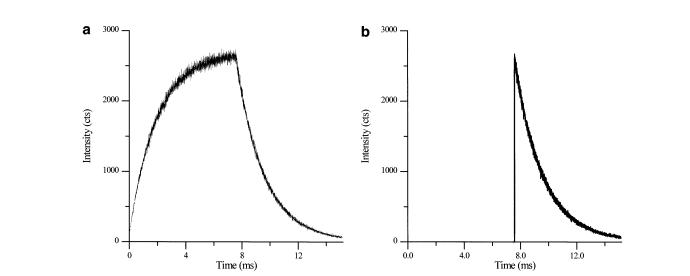
The lifetime of the phosphorescence is able to be calculated from the slope of the decay of the sample after the peak intensity. The lifetime depends on many factors, including the wavelength of the incident radiation as well as properties arising from the sample and the solvent used. Although background fluorescence as well as Raman and Rayleigh scattering are still present in pulsed-time source resolved spectrometry, they are easily detected and removed from intensity versus time plots, allowing for the pure measurement of phosphorescence.
Limitations
The biggest single limitation of molecular phosphorescence spectroscopy is the need for cryogenic conditions. This is a direct result of the unfavorable transition from an excited triplet state to a ground singlet state, which unlikely and therefore produces low-intensity, difficult to detect, long-lasting irradiation. Because cooling phosphorescent samples reduces the chance of other irradiation processes, it is vital for current forms of phosphorescence spectroscopy, but this makes it somewhat impractical in settings outside of a specialized laboratory. However, the emergence and development of room temperature spectroscopy methods give rise to a whole new set of applications and make phosphorescence spectroscopy a more viable method.
Practical Applications
Currently, phosphorescent materials have a variety of uses, and molecular phosphorescence spectrometry is applicable across many industries. Phosphorescent materials find use in radar screens, glow-in-the-dark toys, and in pigments, some of which are used to make highway signs visible to drivers. Molecular phosphorescence spectroscopy is currently in use in the pharmaceutical industry, where its high selectivity and lack of need for extensive separation or purification steps make it useful. It also shows potential in forensic analysis because of the low sample volume requirement.