
1.8: A Practical Introduction to X-ray Absorption Spectroscopy
- Page ID
- 55824

\( \newcommand{\vecs}[1]{\overset { \scriptstyle \rightharpoonup} {\mathbf{#1}} } \)
\( \newcommand{\vecd}[1]{\overset{-\!-\!\rightharpoonup}{\vphantom{a}\smash {#1}}} \)
\( \newcommand{\id}{\mathrm{id}}\) \( \newcommand{\Span}{\mathrm{span}}\)
( \newcommand{\kernel}{\mathrm{null}\,}\) \( \newcommand{\range}{\mathrm{range}\,}\)
\( \newcommand{\RealPart}{\mathrm{Re}}\) \( \newcommand{\ImaginaryPart}{\mathrm{Im}}\)
\( \newcommand{\Argument}{\mathrm{Arg}}\) \( \newcommand{\norm}[1]{\| #1 \|}\)
\( \newcommand{\inner}[2]{\langle #1, #2 \rangle}\)
\( \newcommand{\Span}{\mathrm{span}}\)
\( \newcommand{\id}{\mathrm{id}}\)
\( \newcommand{\Span}{\mathrm{span}}\)
\( \newcommand{\kernel}{\mathrm{null}\,}\)
\( \newcommand{\range}{\mathrm{range}\,}\)
\( \newcommand{\RealPart}{\mathrm{Re}}\)
\( \newcommand{\ImaginaryPart}{\mathrm{Im}}\)
\( \newcommand{\Argument}{\mathrm{Arg}}\)
\( \newcommand{\norm}[1]{\| #1 \|}\)
\( \newcommand{\inner}[2]{\langle #1, #2 \rangle}\)
\( \newcommand{\Span}{\mathrm{span}}\) \( \newcommand{\AA}{\unicode[.8,0]{x212B}}\)
\( \newcommand{\vectorA}[1]{\vec{#1}} % arrow\)
\( \newcommand{\vectorAt}[1]{\vec{\text{#1}}} % arrow\)
\( \newcommand{\vectorB}[1]{\overset { \scriptstyle \rightharpoonup} {\mathbf{#1}} } \)
\( \newcommand{\vectorC}[1]{\textbf{#1}} \)
\( \newcommand{\vectorD}[1]{\overrightarrow{#1}} \)
\( \newcommand{\vectorDt}[1]{\overrightarrow{\text{#1}}} \)
\( \newcommand{\vectE}[1]{\overset{-\!-\!\rightharpoonup}{\vphantom{a}\smash{\mathbf {#1}}}} \)
\( \newcommand{\vecs}[1]{\overset { \scriptstyle \rightharpoonup} {\mathbf{#1}} } \)
\( \newcommand{\vecd}[1]{\overset{-\!-\!\rightharpoonup}{\vphantom{a}\smash {#1}}} \)
\(\newcommand{\avec}{\mathbf a}\) \(\newcommand{\bvec}{\mathbf b}\) \(\newcommand{\cvec}{\mathbf c}\) \(\newcommand{\dvec}{\mathbf d}\) \(\newcommand{\dtil}{\widetilde{\mathbf d}}\) \(\newcommand{\evec}{\mathbf e}\) \(\newcommand{\fvec}{\mathbf f}\) \(\newcommand{\nvec}{\mathbf n}\) \(\newcommand{\pvec}{\mathbf p}\) \(\newcommand{\qvec}{\mathbf q}\) \(\newcommand{\svec}{\mathbf s}\) \(\newcommand{\tvec}{\mathbf t}\) \(\newcommand{\uvec}{\mathbf u}\) \(\newcommand{\vvec}{\mathbf v}\) \(\newcommand{\wvec}{\mathbf w}\) \(\newcommand{\xvec}{\mathbf x}\) \(\newcommand{\yvec}{\mathbf y}\) \(\newcommand{\zvec}{\mathbf z}\) \(\newcommand{\rvec}{\mathbf r}\) \(\newcommand{\mvec}{\mathbf m}\) \(\newcommand{\zerovec}{\mathbf 0}\) \(\newcommand{\onevec}{\mathbf 1}\) \(\newcommand{\real}{\mathbb R}\) \(\newcommand{\twovec}[2]{\left[\begin{array}{r}#1 \\ #2 \end{array}\right]}\) \(\newcommand{\ctwovec}[2]{\left[\begin{array}{c}#1 \\ #2 \end{array}\right]}\) \(\newcommand{\threevec}[3]{\left[\begin{array}{r}#1 \\ #2 \\ #3 \end{array}\right]}\) \(\newcommand{\cthreevec}[3]{\left[\begin{array}{c}#1 \\ #2 \\ #3 \end{array}\right]}\) \(\newcommand{\fourvec}[4]{\left[\begin{array}{r}#1 \\ #2 \\ #3 \\ #4 \end{array}\right]}\) \(\newcommand{\cfourvec}[4]{\left[\begin{array}{c}#1 \\ #2 \\ #3 \\ #4 \end{array}\right]}\) \(\newcommand{\fivevec}[5]{\left[\begin{array}{r}#1 \\ #2 \\ #3 \\ #4 \\ #5 \\ \end{array}\right]}\) \(\newcommand{\cfivevec}[5]{\left[\begin{array}{c}#1 \\ #2 \\ #3 \\ #4 \\ #5 \\ \end{array}\right]}\) \(\newcommand{\mattwo}[4]{\left[\begin{array}{rr}#1 \amp #2 \\ #3 \amp #4 \\ \end{array}\right]}\) \(\newcommand{\laspan}[1]{\text{Span}\{#1\}}\) \(\newcommand{\bcal}{\cal B}\) \(\newcommand{\ccal}{\cal C}\) \(\newcommand{\scal}{\cal S}\) \(\newcommand{\wcal}{\cal W}\) \(\newcommand{\ecal}{\cal E}\) \(\newcommand{\coords}[2]{\left\{#1\right\}_{#2}}\) \(\newcommand{\gray}[1]{\color{gray}{#1}}\) \(\newcommand{\lgray}[1]{\color{lightgray}{#1}}\) \(\newcommand{\rank}{\operatorname{rank}}\) \(\newcommand{\row}{\text{Row}}\) \(\newcommand{\col}{\text{Col}}\) \(\renewcommand{\row}{\text{Row}}\) \(\newcommand{\nul}{\text{Nul}}\) \(\newcommand{\var}{\text{Var}}\) \(\newcommand{\corr}{\text{corr}}\) \(\newcommand{\len}[1]{\left|#1\right|}\) \(\newcommand{\bbar}{\overline{\bvec}}\) \(\newcommand{\bhat}{\widehat{\bvec}}\) \(\newcommand{\bperp}{\bvec^\perp}\) \(\newcommand{\xhat}{\widehat{\xvec}}\) \(\newcommand{\vhat}{\widehat{\vvec}}\) \(\newcommand{\uhat}{\widehat{\uvec}}\) \(\newcommand{\what}{\widehat{\wvec}}\) \(\newcommand{\Sighat}{\widehat{\Sigma}}\) \(\newcommand{\lt}{<}\) \(\newcommand{\gt}{>}\) \(\newcommand{\amp}{&}\) \(\definecolor{fillinmathshade}{gray}{0.9}\)X-ray absorption spectroscopy (XAS) is a technique that uses synchrotron radiation to provide information about the electronic, structural, and magnetic properties of certain elements in materials. This information is obtained when X-rays are absorbed by an atom at energies near and above the core level binding energies of that atom. Therefore, a brief description about X-rays, synchrotron radiation and X-ray absorption is provided prior to a description of sample preparation for powdered materials.
X-rays and Synchrotron Radiation
X-rays were discovered by the Wilhelm Röntgen in 1895 (figure \(\PageIndex{1}\)). They are a form of electromagnetic radiation, in the same manner as visible light but with a very short wavelength, around 0.25 - 25 Å. As electromagnetic radiation, X-rays have a specific energy. The characteristic range is defined by soft versus hard X-rays. Soft X-rays cover the range from hundreds of eV to a few KeV, and the hard X-rays have an energy range from a few KeV up to around 100 KeV.
X-rays are commonly produced by X-ray tubes, when high-speed electrons strike a metal target. The electrons are accelerated by a high voltage towards the metal target; X-rays are produced when the electrons collide with the nuclei of the metal target.
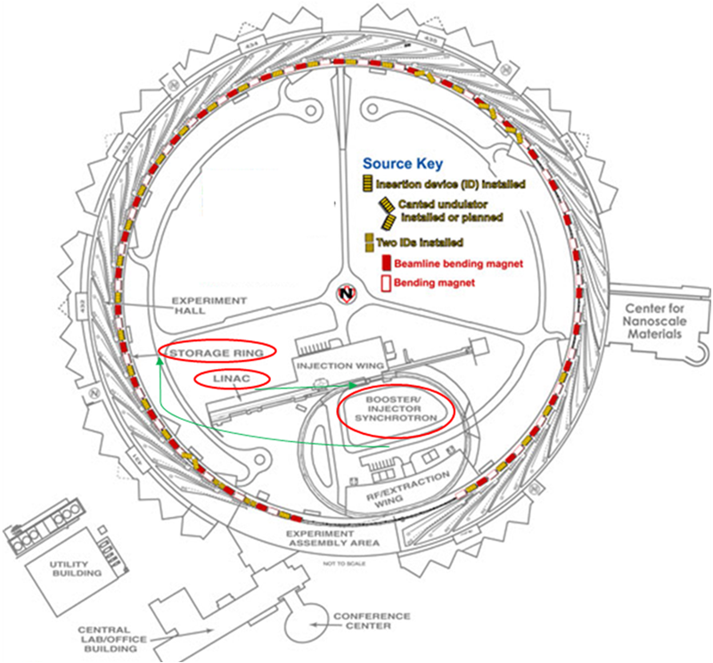
Synchrotron radiation is generated when particles are moving at really high velocities and are deflected along a curved trajectory by a magnetic field. The charged particles are first accelerated by a linear accelerator (LINAC) (figure \(\PageIndex{2}\)); then, they are accelerated in a booster ring that injects the particles moving almost at the speed of light into the storage ring. There, the particles are accelerated toward the center of the ring each time their trajectory is changed so that they travel in a closed loop. X-rays with a broad spectrum of energies are generated and emitted tangential to the storage ring. Beamlines are placed tangential to the storage ring to use the intense X-ray beams at a wavelength that can be selected varying the set up of the beamlines. Those are well suited for XAS measurements because the X-ray energies produced span 1000 eV or more as needed for an XAS spectrum.
X-ray Absorption
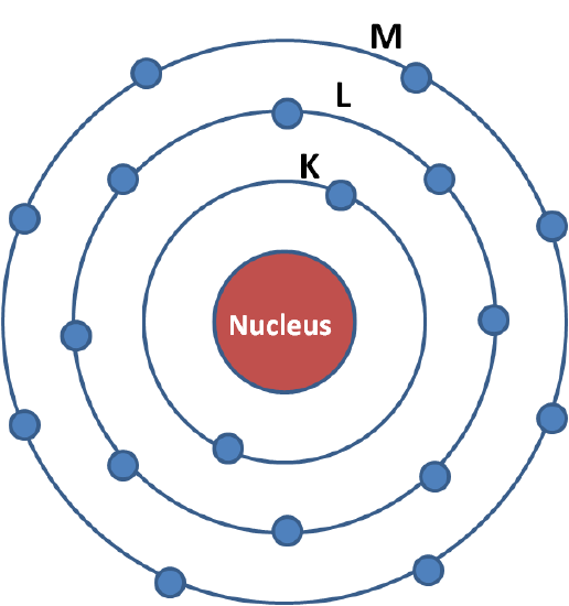
Light is absorbed by matter through the photoelectric effect. It is observed when an X-ray photon is absorbed by an electron in a strongly bound core level (such as the 1s or 2p level) of an atom (figure \(\PageIndex{3}\)). In order for a particular electronic core level to participate in the absorption, the binding energy of this core level must be less than the energy of the incident X-ray. If the binding energy is greater than the energy of the X-ray, the bound electron will not be perturbed and will not absorb the X-ray. If the binding energy of the electron is less than that of the X-ray, the electron may be removed from its quantum level. In this case, the X-ray is absorbed and any energy in excess of the electronic binding energy is given as kinetic energy to a photo-electron that is ejected from the atom.
When X-ray absorption is discussed, the primary concern is about the absorption coefficient, µ, which gives the probability that X-rays will be absorbed according to Beer’s Law where I0 is the X-ray intensity incident on a sample, t is the sample thickness, and I is the intensity transmitted through the sample.
\[I = I _ { 0 } e ^ { - \mu t } \label{eq:BeerLambert} \]
The absorption coefficient, µE, is a smooth function of energy, with a value that depends on the sample density ρ, the atomic number Z, atomic mass A, and the X-ray energy E roughly as
\[ \mu _ { E } \approx \frac { \rho Z ^ { 4 } } { A E ^ { 3 } } \nonumber \]
When the incident X-ray has energy equal to that of the binding energy of a core-level electron, there is a sharp rise in absorption: an absorption edge corresponding to the promotion of this core level to the continuum. For XAS, the main concern is the intensity of µ, as a function of energy, near and at energies just above these absorption edges. An XAS measurement is simply a measure of the energy dependence of µ at and above the binding energy of a known core level of a known atomic species. Since every atom has core-level electrons with well-defined binding energies, the element to probe can be selected by tuning the X-ray energy to an appropriate absorption edge. These absorption edge energies are well-known. Because the element of interest is chosen in the experiment, XAS is element-specific.
X-ray Absorption Fine Structure
X-ray absorption fine structure (XAFS) spectroscopy, also named X-ray absorption spectroscopy, is a technique that can be applied for a wide variety of disciplines because the measurements can be performed on solids, gasses, or liquids, including moist or dry soils, glasses, films, membranes, suspensions or pastes, and aqueous solutions. Despites its broad adaptability with the kind of material used, there are samples which limits the quality of an XAFS spectrum. Because of that, the sample requirements and sample preparation is reviewed in this section as well the experiment design which are vital factors in the collection of good data for further analysis.
Experiment Design
The main information can be obtained using XAFS spectra consist in small changes in the absorption coefficient (E), which can be measured directly in a transmission mode or indirectly using a fluorescence mode. Therefore, a good signal to noise ratio is required (better than 103). In order to obtain this signal to noise ratio, an intense beam is required (on the order 1010 photons/second or better), with the energy bandwidth of 1 eV or less, and the capability of scanning the energy of the incident beam over a range of about 1 KeV above the edge in a time range of seconds or few minutes. As a result, synchrotron radiation is preferred further than other kind of X-ray sources previously mentioned.
Beamline Setup
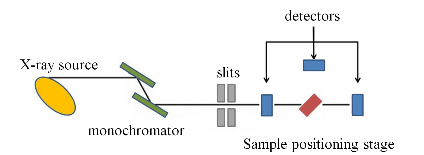
Despite the setup of a synchrotron beamline is mostly done by the assistance of specialist beamline scientists, nevertheless, it is useful to understand the system behind the measurement. The main components of a XAFS beamline, as shown in figure below, are as follows:
- A harmonic rejection mirror to reduce the harmonic content of the X-ray beam.
- A monochromator to choose the X-ray energy.
- A series of slits which defines the X-ray profile.
- A sample positioning stage.
- The detectors, which can be a single ionization detector or a group of detectors to measure the X-ray intensity.
Slits are used to define the X-ray beam profile and to block unwanted X-rays. Slits can be used to increase the energy resolution of the X-ray incident on the sample at the expense of some loss in X-ray intensity. They are either fixed or adjustable slits. Fixed slits have a pre-cut opening of heights between 0.2 and 1.0 mm and a width of some centimeters. Adjustable slits use metal plates that move independently to define each edge of the X-ray beam.
Monochromator
The monochromator is used to select the X-ray energy incident on the sample. There are two main kinds of X-ray monochromators:
- The double-crystal monochromator, which consists of two parallel crystals.
- The channel-cut monochromator, which is a single crystal with a slot cut nearly through it.
Most monochromator crystals are made of silicon or germanium and are cut and polished such that a particular atomic plane of the crystal is parallel to the surface of the crystal as Si(111), Si(311), or Ge(111). The energy of X-rays diffracted by the crystal is controlled by rotating the crystals in the white beam.
Harmonic rejection mirrors
The harmonic X-ray intensity needs to be reduced, as these X-rays will adversely affect the XAS measurement. A common method for removing harmonic X-rays is using a harmonic rejection mirror. This mirror is usually made of Si for low energies, Rh for X-ray energies below the Rh absorption edge at 23 keV, or Pt for higher X-ray energies. The mirror is placed at a grazing angle in the beam such that the X-rays with fundamental energy are reflected toward the sample, while the harmonic X-rays are not.
Detectors
Most X-ray absorption measurements use ionization detectors. These contain two parallel plates separated by a gas-filled space that the X-rays travel through. Some of the X-rays ionize the gas particles. A voltage bias applied to the parallel plates separates the gas ions, creating a current. The applied voltage should give a linear detector response for a given change in the incident X-ray intensity. There are also other kinds as fluorescence and electron yield detectors.
Transmission and Fluorescence Modes
X-ray Absorption measurements can be performed in several modes: transmission, fluorescence and electron yield; where the two first are the most common. The choice of the most appropriate mode to use in one experiment is a crucial decision.
The transmission mode is the most used because it only implies the measure of the X-ray flux before and after the beam passes the sample. Therefore, the adsorption coefficient is defined as
\[ \mu _ { E } = \ln \left( \frac { I _ { 0 } } { I } \right) \nonumber \]
Transmission experiments are standard for hard X-rays, because the use of soft X-rays implies the use the samples thinner than 1 μm. Also, this mode should be used for concentrated samples. The sample should have the right thickness and be uniform and free of pinholes.
The fluorescence mode measures the incident flux I0 and the fluorescence X-rays If that are emitted following the X-ray absorption event. Usually the fluorescent detector is placed at 90° to the incident beam in the horizontal plane, with the sample at an angles, commonly 45°, with respect to the beam, because in that position there is not interference generated because of the initial X-ray flux (I0). The use of fluorescence mode is preferred for thicker samples or lower concentrations, even ppm concentrations or lower. For a highly concentrated sample, the fluorescence X-rays are reabsorbed by the absorber atoms in the sample, causing an attenuation of the fluorescence signal, it effect is named as self-absorption and is one of the most important concerns in the use of this mode.
Sample Preparation for XAS
Sample Requirements
Uniformity
The samples should have a uniform distribution of the absorber atom, and have the correct absorption for the measurement. The X-ray beam typically probes a millimeter-size portion of the sample. This volume should be representative of the entire sample.
Thickness
For transmission mode samples, the thickness of the sample is really important. It supposes to be a sample with a given thickness, t, where the total adsorption of the atoms is less than 2.5 adsorption lengths, µEt ≈ 2.5; and the partial absorption due to the absorber atoms is around one absorption length ∆ µEt ≈ 1, which corresponds to the step edge.
The thickness to give ∆ µEt = 1 is as
\[t = \frac { 1 } { \Delta \mu } = \frac { 1.66 \sum _ { i } n _ { i } M _ { i } } { \rho \sum _ { i } n _ { i } \left[ \sigma _ { i } \left( E _ { + } \right) - \sigma _ { i } \left( E _ { - } \right) \right] } \nonumber \]
where ρ is the compound density, n is the elemental stoichiometry, M is the atomic mass, σE is the adsorption cross-section in barns/atom (1 barn = 10-24 cm2) tabulated in McMaster tables, and E+and E- are the just above and below the energy edge. This calculation can be accomplished using the free download software HEPHAESTUS.
Total X-ray Adsorption
For non-concentrate samples, the total X-ray adsorption of the sample is the most important. It should be related to the area concentration of the sample (\(ρt\), in g/cm2). The area concentration of the sample multiplied by the difference of the mass adsorption coefficient (\(∆µE/ρ\)) give the edge step, where a desired value to obtain a good measure is a edge step equal to one, \((∆µE/ρ)ρt ≈ 1\).
The difference of the mass adsorption coefficient is given by
\[ \left( \frac { \Delta \mu _ { E } } { \rho } \right) = \sum f _ { i } \left[ \left( \frac { \Delta \mu _ { E } } { \rho } \right) _ { i , ( E_+ ) } - \left( \frac { \Delta \mu _ { E } } { \rho } \right) _ { i , \left( E _{ - } \right) } \right] \nonumber \]
where \((µE/ρ)_i \) is the mass adsorption coefficient just above (\(E_+\)) and below (\(E_-\)) of the edge energy and \(f_i\) is the mass fraction of the element i. Multiplying the area concentration, \(ρt\), for the cross-sectional area of the sample holder, amount of sample needed is known.
Sample Preparation
As was described in last section, there are diluted solid samples, which can be prepared onto big substrates or concentrate solid samples which have to be prepared in thin films. Both methods are following described.
Liquid and gases samples can also be measured, but the preparation of those kind of sample is not discussed in this paper because it depends in the specific requirements of each sample. Several designs can be used as long they avoid the escape of the sample and the material used as container does not absorb radiation at the energies used for the measure.
Method 1
- The materials needed are showed in this figure: Kapton tape and film, a thin spatula, tweezers, scissors, weigh paper, mortar and pestle, and a sample holder. The sample holder can be made from several materials, as polypropylene, polycarbonate or Teflon.
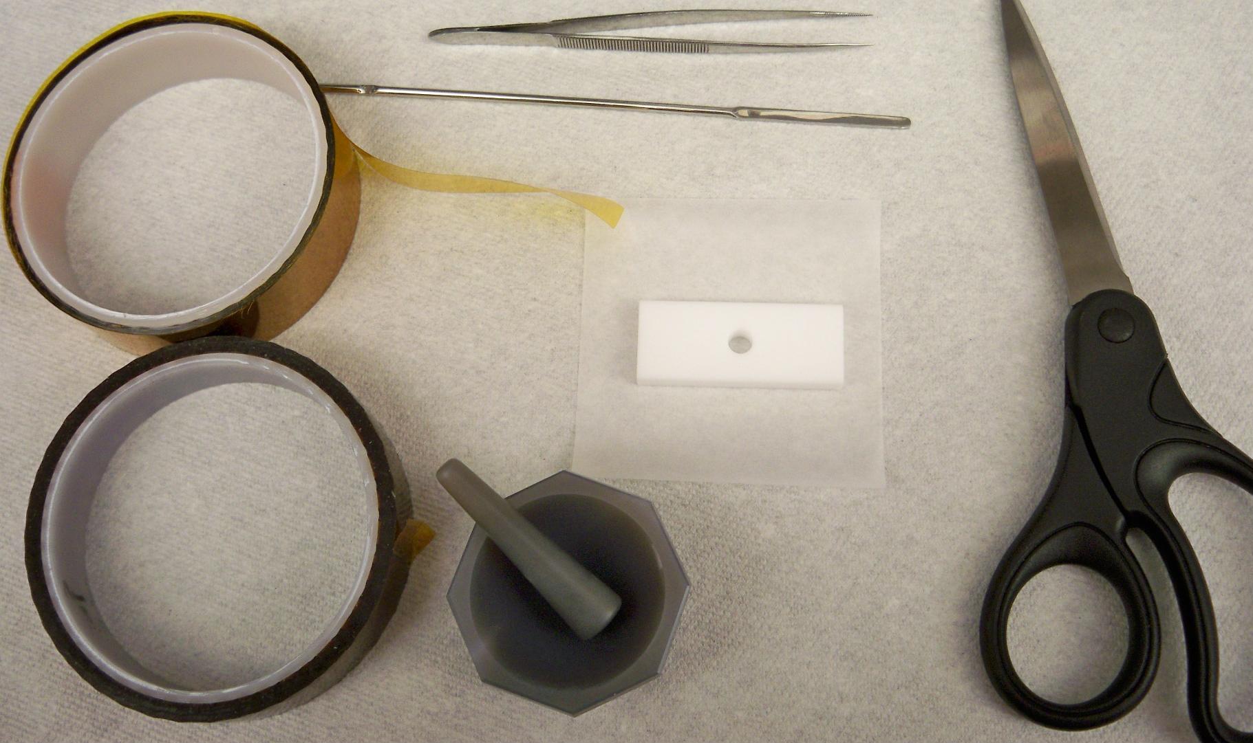
Figure \(\PageIndex{5}\): Several tools are needed for the sample preparation using Method 1. - Two small squares of Kapton film are cut. One of them is placed onto the hole of the sample holder as shown figure \(\PageIndex{6}\)a. A piece of Kapton tape is placed onto the sample holder trying to minimize any air burble onto the surface and keeping the film as was previously placed figure \(\PageIndex{6}\)b. A side of the sample holder is now sealed in order to fill the hole (figure \(\PageIndex{7}\)).
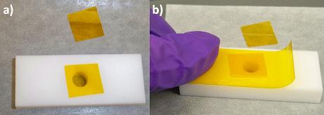
Figure \(\PageIndex{6}\): Preparing one face of the sample holder by (a) positioning a small piece of Kapton film onto the hole, which is held in place by Kapton tape (b). 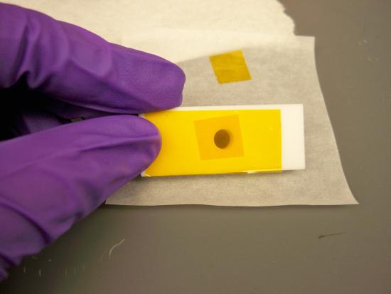
Figure \(\PageIndex{7}\): The side of the sample holder is closed. - Before fill the sample holder, make sure your sample is a fine powder. Use the mortar to grind the sample.
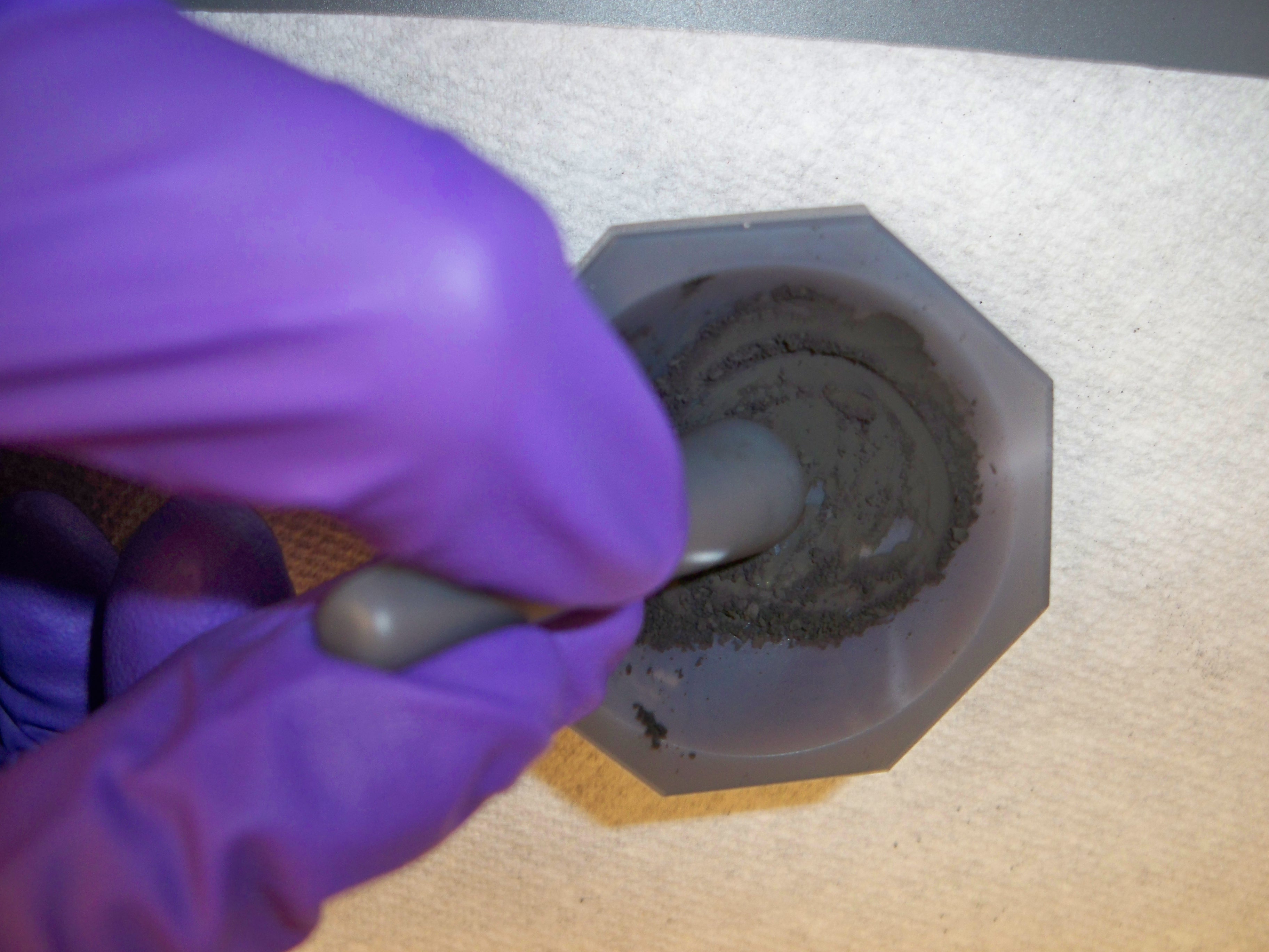
Figure \(\PageIndex{8}\): The sample is ground to be sure the grain size of the sample is homogeneous and small enough. - Fill the hole with the powder. Make sure you have extra powder onto the hole (figure \(\PageIndex{9}\)a). With the spatula press the powder. The sample has to be as compact as possible (figure \(\PageIndex{9}\)b).
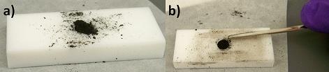
Figure \(\PageIndex{9}\): The sample holder is filled by (a) adding extra powder onto the hole then (b) compacting the sample with the spatula. - Clean the surface of the slide. Repeat the step 2. Your sample loaded in the sample holder should look as picture below:
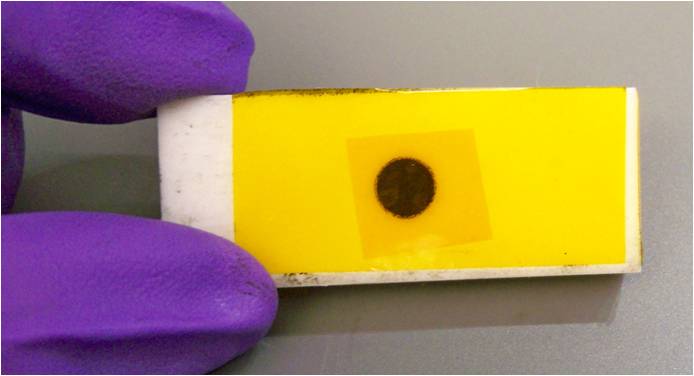
Figure \(\PageIndex{10}\): Sample loaded and sealed into the sample holder.
Method 2
- The materials needed are showed in photo: Kapton tape, tweezers, scissors, weigh paper, mortar and pestle, tape and aluminum foil.
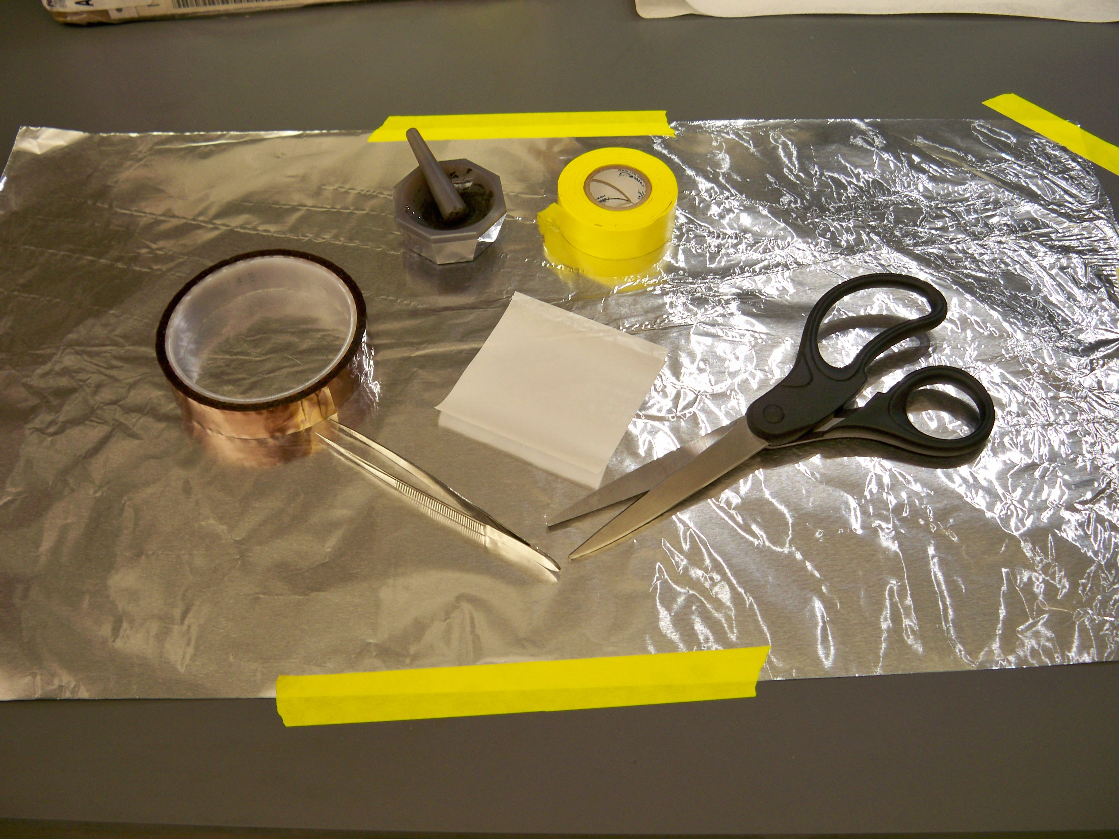
Figure \(\PageIndex{11}\): Several utensils are needed for the sample preparation using Method 2. - Aluminum foil is placed as the work-area base. Kapton tape is place from one corner to the opposite one as shown figure \(\PageIndex{12}\). Tape is put onto the extremes to fix it. In this case yellow tape was used in order to show where the tape should be placed but is better use Scotch invisible tape for the following steps.
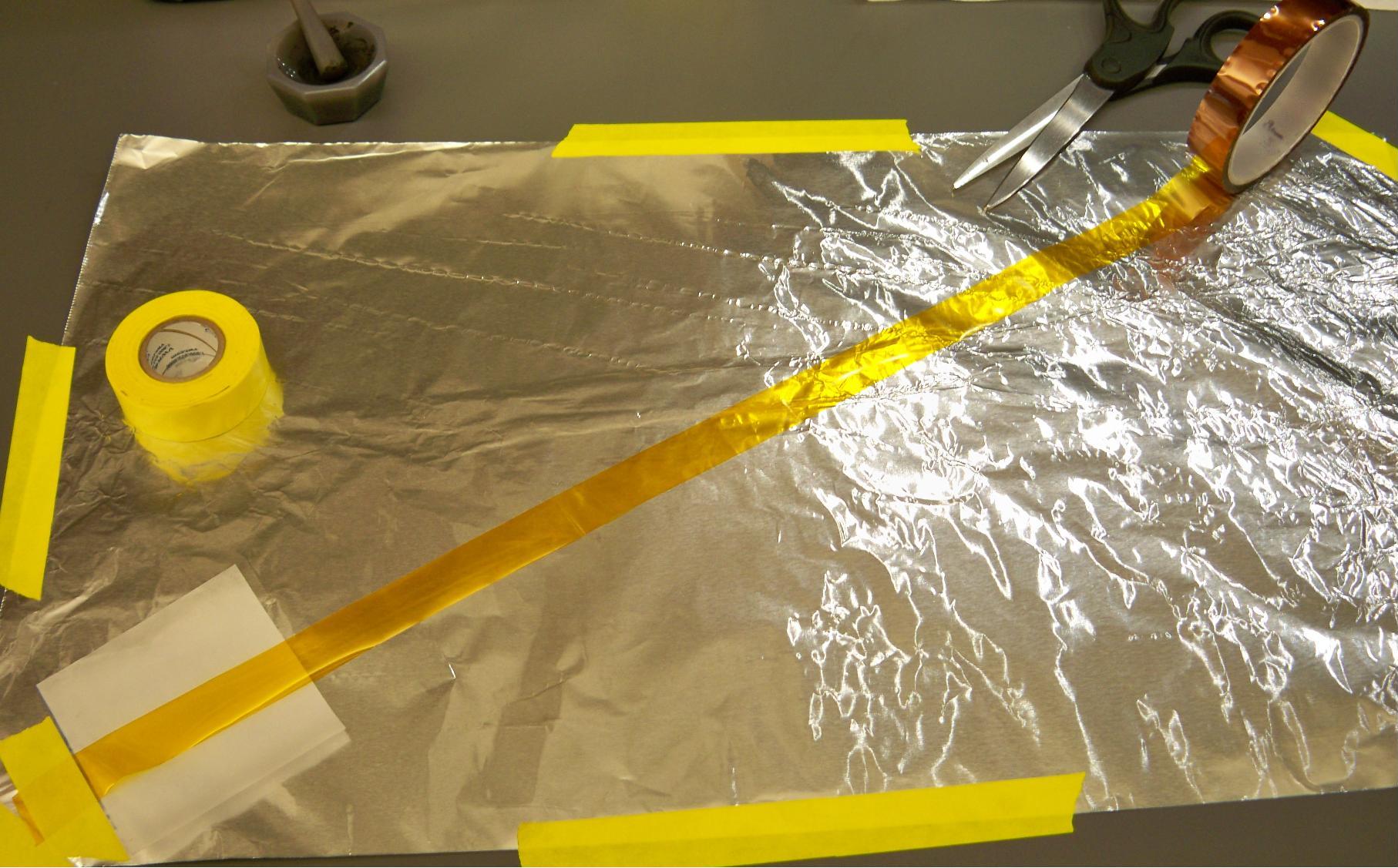
Figure \(\PageIndex{12}\): Preparation of the work-area. - The weigh paper is placed under the Kapton tape in one of the extremes. Sample is added onto that Kapton tape extreme. The function of the weigh paper is further recuperation of extra sample.
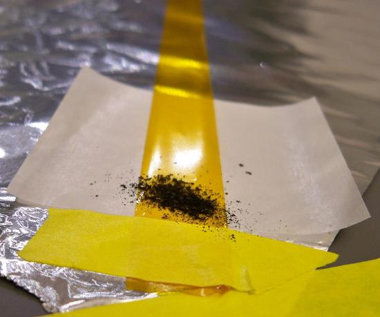
Figure \(\PageIndex{13}\): Add the sample onto an extreme of the Kapton tape. - With one finger, the sample is dispersed along the Kapton tape, always in the same direction and taking care that the weigh paper is under the tape area is being used (figure \(\PageIndex{14}\)a). The finger should be slid several times making pressure in order to have a homogeneous and complete cover film (figure \(\PageIndex{14}\)b).

Figure \(\PageIndex{14}\): Making a thin film with a solid sample by (a) dispersing the solid along the Kapton tape and (b) repeated sliding several times to obtain a homogeneous film. - The final sample covered Kapton tape should look like figure \(\PageIndex{15}\). Cut the extremes in order to a further manipulation of the film.
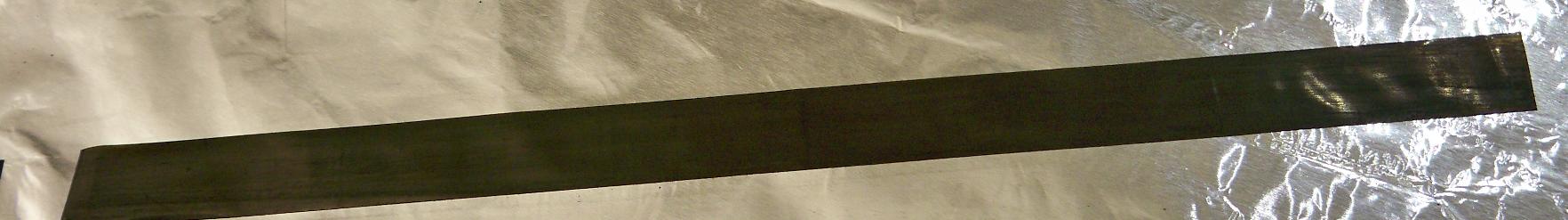
Figure \(\PageIndex{15}\): A complete thin film. - Using the tweezers, fold the film taking care that is well aligned and there fold is complete plane. figure \(\PageIndex{16}\)a shows the first folding, generating a 2 layers film. figure \(\PageIndex{16}\)b and figure \(\PageIndex{16}\)c shows the second and third folding, obtaining a 4 and 8 layers film. Sometimes a 4 layers film is good enough. You always can fold again to obtain bigger signal intensity.
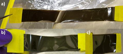
Figure \(\PageIndex{16}\): Folding of the thin film simple once results in a two layer film (a) and after a second and third folding four and eight layers films are obtained (b and c, respectively).
Bibliography
- B. D. Cullity and S. R. Stock. Elements of X-ray Diffraction, Prentice Hall, Upper Saddle River (2001).
- F. Hippert, E. Geissler, J. L. Hodeau, E. Lelièvre-Berna, and J. R. Regnard. Neutron and X-ray Spectroscopy, Springer, Dordrecht (2006).
- G. Bunker. Introduction to XAFS: A practical guide to X-ray Absorption Fine Structure Spectroscopy, Cambridge University Press, Cambridge (2010).
- S. D. Kelly, D. Hesterberg, and B. Ravel in Methods of Soil Analysis: Part 5, Mineralogical Methods, Ed. A. L. Urely and R. Drees, Soil Science Society of America Book Series, Madison (2008).