1.3: Introduction to Combustion Analysis

Applications of Combustion Analysis

Combustion, or burning as it is more commonly known, is simply the mixing and exothermic reaction of a fuel and an oxidizer. It has been used since prehistoric times in a variety of ways, such as a source of direct heat, as in furnaces, boilers, stoves, and metal forming, or in piston engines, gas turbines, jet engines, rocket engines, guns, and explosives. Automobile engines use internal combustion in order to convert chemical into mechanical energy. Combustion is currently utilized in the production of large quantities of \(\ce{H2}\). Coal or coke is combusted at 1000^◦C in the presence of water in a two-step reaction. The first step shown in involved the partial oxidation of carbon to carbon monoxide.

\[\ce{C(g) + H2O(g) -> CO(g) + H2(g)} \nonumber \]

The second step involves a mixture of produced carbon monoxide with water to produce hydrogen and is commonly known as the water gas shift reaction.

\[\ce{CO(g) + H2O(g) → CO2(g) + H2(g)} \nonumber \]

Although combustion provides a multitude of uses, it was not employed as a scientific analytical tool until the late 18^th century.

History of Combustion

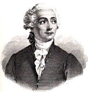
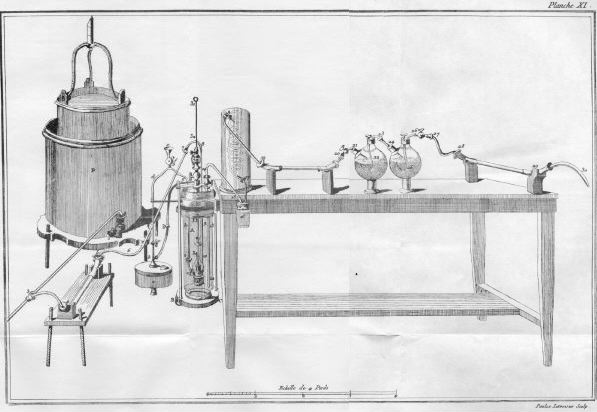
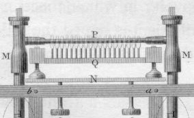
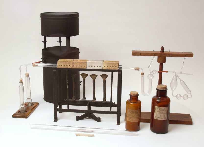
In the 1780's, Antoine Lavoisier (figure \(\PageIndex{1}\) ) was the first to analyze organic compounds with combustion using an extremely large and expensive apparatus (figure \(\PageIndex{2}\) ) that required over 50 g of the organic sample and a team of operators.

Figure \(\PageIndex{1}\): French chemist and renowned "father of modern Chemistry" Antoine Lavoisier (1743-1794).

Figure \(\PageIndex{2}\): Lavoisier's combustion apparatus. A. Lavoisier, Traité Élémentaire de Chimie, 1789, 2, 493-501.

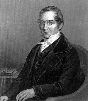
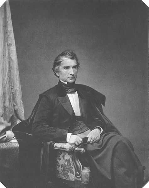
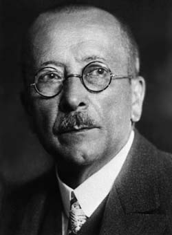
The method was simplified and optimized throughout the 19^th and 20^th centuries, first by Joseph Gay- Lussac (Figure \(\PageIndex{3}\)), who began to use copper oxide in 1815, which is still used as the standard catalyst.

Figure \(\PageIndex{3}\): French chemist Joseph Gay-Lussac (1778-1850).

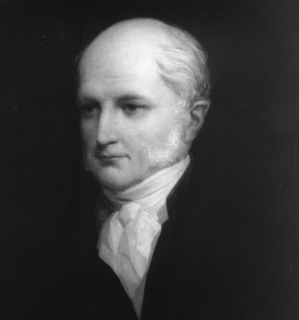
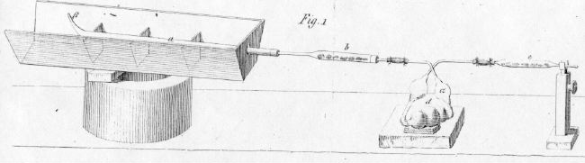
William Prout (Figure \(\PageIndex{4}\)) invented a new method of combustion analysis in 1827 by heating a mixture of the sample and \(\ce{CuO }\) using a multiple-flame alcohol lamp (Figure \(\PageIndex{5}\)) and measuring the change in gaseous volume.

Figure \(\PageIndex{4}\): English chemist, physician, and natural theologian William Prout (1785-1850).

Figure \(\PageIndex{5}\): Prout's combustion apparatus. W. Prout, Philos. T. R. Soc. Lond., 1827, 117, 355.

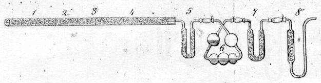
In 1831, Justus von Liebig (Figure \(\PageIndex{6}\))) simplified the method of combustion analysis into a "combustion train" system (Figure \(\PageIndex{7}\)) and Figure \(\PageIndex{8}\))) that linearly heated the sample using coal, absorbed water using calcium chloride, and absorbed carbon dioxide using potash (KOH). This new method only required 0.5 g of sample and a single operator, and Liebig moved the sample through the apparatus by sucking on an opening at the far right end of the apparatus.

Figure \(\PageIndex{6}\): German chemist Justus von Liebig (1803-1873).

Figure \(\PageIndex{7}\): Print of von Liebig's "combustion train" apparatus for determining carbon and hydrogen composition. J. Von Liebig, Annalen der Physik und Chemie, 1831, 21.

Figure \(\PageIndex{8}\): Photo of von Liebig's "combustion train apparatus" for determining carbon and hydrogen composition. The Oesper Collections in the History of Chemistry, Apparatus Museum, University of Cincinnati, Case 10, Combustion Analysis. For a 360^o view of this apparatus, click here.

Jean-Baptiste André Dumas (Figure \(\PageIndex{9}\))) used a similar combustion train to Liebig. However, he added a U-shaped aspirator that prevented atmospheric moisture from entering the apparatus (Figure \(\PageIndex{10}\))).

Figure \(\PageIndex{9}\): French chemist Jean-Baptiste André Dumas (1800-1844).

Figure \(\PageIndex{10}\): Dumas' apparatus; note the aspirator at 8. Sourced from J. A. Dumas, Ann. der Chem. and Pharm., 1841, 38, 141.

In 1923, Fritz Pregl (Figure \(\PageIndex{11}\))) received the Nobel Prize for inventing a micro-analysis method of combustion. This method required only 5 mg or less, which is 0.01% of the amount required in Lavoisier's apparatus.

Figure \(\PageIndex{11}\): Austrian chemist and physician Fritz Pregl (1869-1930).

Today, combustion analysis of an organic or organometallic compound only requires about 2 mg of sample. Although this method of analysis destroys the sample and is not as sensitive as other techniques, it is still considered a necessity for characterizing an organic compound.

Categories of combustion

Basic flame types

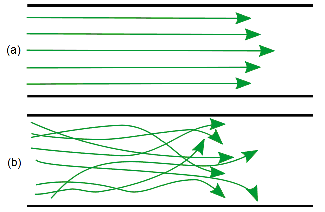
There are several categories of combustion, which can be identified by their flame types (Table \(\PageIndex{1}\)). At some point in the combustion process, the fuel and oxidant must be mixed together. If these are mixed before being burned, the flame type is referred to as a premixed flame, and if they are mixed simultaneously with combustion, it is referred to as a nonpremixed flame. In addition, the ow of the flame can be categorized as either laminar (streamlined) or turbulent (Figure \(\PageIndex{12}\)).

Table \(\PageIndex{1}\): Types of combustion systems with examples. Adapted from J. Warnatz, U. Maas, and R. W. Dibble, Combustion: Physical and Chemical Fundamentals, Modeling and Simulation, Experiments, Pollutant Formation, 3rd Ed., Springer, Berlin (2001).

Fuel/oxidizer mixing	Fluid motion	Examples
Premixed	Turbulent	Spark-ignited gasoline engine, low NOx stationary gas turbine
Premixed	Laminar	Flat flame, Bunsen flame (followed by a nonpremixed candle for Φ>1)
Nonpremixed	Turbulent	Pulverized coal combustion, aircraft turbine, diesel engine, H2/O2 rocket motor
Nonpremixed	Laminar	Wood fire, radiant burners for heating, candle

Figure \(\PageIndex{12}\): Schematic representation of (a) laminar flow and (b) turbulent flow.

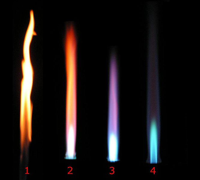
The amount of oxygen in the combustion system can alter the ow of the flame and the appearance. As illustrated in Figure \(\PageIndex{13}\), a flame with no oxygen tends to have a very turbulent flow, while a flame with an excess of oxygen tends to have a laminar flow.

Figure \(\PageIndex{13}\): Bunsen burner flames with varying amounts of oxygen and constant amount of fuel. (1) air valve completely closed, (2) air valve slightly open, (3) air valve half open, (4) air valve completely open.

Stoichiometric combustion and calculations

A combustion system is referred to as stoichiometric when all of the fuel and oxidizer are consumed and only carbon dioxide and water are formed. On the other hand, a fuel-rich system has an excess of fuel, and a fuel-lean system has an excess of oxygen (Table \(\PageIndex{2}\)).

Table \(\PageIndex{2}\): Examples of stoichiometric, fuel-rich, and fuel-lean systems.

Combustion type	Reaction example
Stoichiometric	\(\ce{2H2 + O2 -> 2H2O}\)
Fuel-rich (\(\ce{H2}\) left over)	\(\ce{3H2 +O2 ->2H2O+H2}\)
Fuel-lean (\(\ce{O2}\) left over)	\(\ce{CH4 +3O2 ->2H2O+CO2 +O2}\)

If the reaction of a stoichiometric mixture is written to describe the reaction of exactly 1 mol of fuel (\(\ce{H2}\) in this case), then the mole fraction of the fuel content can be easily calculated as follows, where \( ν \) denotes the mole number of \(\ce{O2}\) in the combustion reaction equation for a complete reaction to \(\ce{H2O}\) and \(\ce{CO2}\),

\[ x_{\text{fuel, stoich}} = \dfrac{1}{1+v} \nonumber \]

For example, in the reaction

\[\ce{H2 + 1/2 O2 → H2O2 + H2} \nonumber \]

we have \( v = \frac{1}{2} \), so the stoichiometry is calculated as

\[ x_{\ce{H2}, \text{stoich}}= \dfrac{1}{1+0.5} = 2/3 \nonumber \]

However, as calculated this reaction would be for the reaction in an environment of pure oxygen. On the other hand, air has only 21% oxygen (78% nitrogen, 1% noble gases). Therefore, if air is used as the oxidizer, this must be taken into account in the calculations, i.e.

\[ x_{\ce{N2}} = 3.762 (x_{\ce{O2}}) \nonumber \]

The mole fractions for a stoichiometric mixture in air are therefore calculated in following way:

\[ x_{\text{fuel, stoich}} = \dfrac{1}{1+v(4.762)} \label{eq:xfuel} \]

\[ x_{\ce{O2},\text{stoich}} = v(x_{\text{fuel, stoich}}) \nonumber \]

\[ x_{\ce{N2},\text{stoich}} = 3.762(x_{\ce{O2}, \text{stoich}}) \nonumber \]

Example \(\PageIndex{1}\):

Calculate the fuel mole fraction (\(x_{\text{fuel}} \)) for the stoichiometric reaction:

\[ \ce{CH4 + 2O2} + (2 \times 3.762)\ce{N2 → CO2 + 2H2O} + (2 \times 3.762)\ce{N2} \nonumber \]

Solution

In this reaction \( ν \) = 2, as 2 moles of oxygen are needed to fully oxidize methane into \(\ce{H2O}\) and
\(\ce{CO2}\).

\[ x_{\text{fuel, stoich}} = \dfrac{1}{1+2 \times 4.762} = 0.09502 = 9.502~\text{mol} \% \nonumber \]

Exercise \(\PageIndex{1}\)

Calculate the fuel mole fraction for the stoichiometric reaction:

\[ \ce{C3H8 + 5O2} + (5 \times 3.762)\ce{N2 → 3CO2 + 4H2O} + (5 \times 3.762)\ce{N2} \nonumber \]

Answer

The fuel mole fraction is 4.03%

Premixed combustion reactions can also be characterized by the air equivalence ratio, \( \lambda \):

\[ \lambda = \dfrac{x_{\text{air}}/x_{\text{fuel}}}{x_{\text{air, stoich}}/x_{\text{fuel,stoich}}} \nonumber \]

The fuel equivalence ratio, \( Φ\), is the reciprocal of this value

\[ Φ = 1/\lambda \nonumber \]

Rewriting \ref{eq:xfuel} in terms of the fuel equivalence ratio gives:

\[ x_{\text{fuel}} = \frac { 1 } { 1 + v( 4.672 / \Phi ) } \nonumber \]

\[ x_{\text{air}} = 1 - x_{\text{fuel}} \nonumber \]

\[ x_{\ce{O2}} = x_{\text{air}}/4.762 \nonumber \]

\[ x_{\ce{N2}} = 3.762(x_{\ce{O2}}) \nonumber \]

The premixed combustion processes can also be identified by their air and fuel equivalence ratios (Table \(\PageIndex{3}\) ).

Table \(\PageIndex{3}\): Identification of combustion type by Φ and λ values.

Type of combustion	Φ	λ
Rich	>1	<1
Stoichiometric	=1	=1
Lean	<1	>1

With a premixed type of combustion, there is much greater control over the reaction. If performed at lean conditions, then high temperatures, the pollutant nitric oxide, and the production of soot can be minimized or even avoided, allowing the system to combust efficiently. However, a premixed system requires large volumes of premixed reactants, which pose a fire hazard. As a result, nonpremixed combusted, while not being efficient, is more commonly used.

Instrumentation

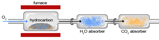
Though the instrumentation of combustion analysis has greatly improved, the basic components of the apparatus (Figure 1.14) have not changed much since the late 18^th century.

Figure \(\PageIndex{14}\) : Combustion apparatus from the 19^th century. The Oesper Collections in the History of Chemistry Apparatus Museum, University of Cincinnati, Case 10, Combustion Analysis. For a 360^o view of this apparatus, click here.

The sample of an organic compound, such as a hydrocarbon, is contained within a furnace or exposed to a ame and burned in the presence of oxygen, creating water vapor and carbon dioxide gas (Figure \(\PageIndex{15}\)). The sample moves first through the apparatus to a chamber in which\(\ce{H2O}\) is absorbed by a hydrophilic substance and second through a chamber in which \(\ce{CO2}\) is absorbed. The change in weight of each chamber is determined to calculate the weight of \(\ce{H2O}\) and \(\ce{CO2}\). After the masses of \(\ce{H2O}\) and \(\ce{CO2}\) have been determined, they can be used to characterize and calculate the composition of the original sample.

Figure \(\PageIndex{15}\): Typical modern combustion apparatus with a furnace.

Calculations and determining chemical formulas

Hydrocarbons

Combustion analysis is a standard method of determining a chemical formula of a substance that contains hydrogen and carbon. First, a sample is weighed and then burned in a furnace in the presence of excess oxygen. All of the carbon is converted to carbon dioxide, and the hydrogen is converted to water in this way. Each of these are absorbed in separate compartments, which are weighed before and after the reaction. From these measurements, the chemical formula can be determined.

Generally, the following reaction takes place in combustion analysis:

\[ \ce{C_{a}H_{b} + O2(xs) → aCO2 + b/2 H2O} \nonumber \]

Example \(\PageIndex{2}\):

After burning 1.333 g of a hydrocarbon in a combustion analysis apparatus, 1.410 g of \(\ce{H2O}\) and 4.305 g of \(\ce{CO2}\) were produced. Separately, the molar mass of this hydrocarbon was found to be 204.35 g/mol. Calculate the empirical and molecular formulas of this hydrocarbon.

Step 1: Using the molar masses of water and carbon dioxide, determine the moles of hydrogen and carbon that were produced.

\[ 1.410~\text{g}~\ce{H2O} \times \dfrac{1~\text{mol}~\ce{H2O}}{18.015~\text{g}~\ce{H2O}} \times \dfrac{2~\text{mol H}}{1~\text{mol}~\ce{H2O}} = 0.1565~\text{mol H} \nonumber \]

\[ 4.3051~\text{g}~\ce{CO2} \times \dfrac{1~\text{mol}~\ce{CO2}}{44.010~\text{g}~\ce{CO2}} \times \dfrac{1~\text{mol C}}{1~\text{mol}~\ce{CO2}} = 0.09782 ~\text{mol C} \nonumber \]

Step 2: Divide the larger molar amount by the smaller molar amount. In some cases, the ratio is not made up of two integers. Convert the numerator of the ratio to an improper fraction and rewrite the ratio in whole numbers as shown

\[ \frac { 0.1565~\mathrm { mol~H } } { 0.09782~\mathrm{ mol~C} } = \frac { 1.600~\mathrm { mol~H } } { 1~\mathrm { mol~C } } = \frac { 16 / 10~\mathrm { mol~H } } { 1~\mathrm { mol~C } } = \frac { 8 / 5~\mathrm { mol~H } } { 1~\mathrm { mol~C } } = \frac { 8~\mathrm { mol~H } } { 5~\mathrm { mol~C } } \nonumber \]

Therefore, the empirical formula is \(\ce{C5H8}\).

Step 3: To get the molecular formula, divide the experimental molar mass of the unknown hydrocarbon by the empirical formula weight.

\[ \frac { \text { Molar mass } } { \text { Empirical formula weight } } = \frac { 204.35~\mathrm { g } / \mathrm { mol } } { 68.114~\mathrm { g } / \mathrm { mol } } = 3 \nonumber \]

Therefore, the molecular formula is \(\ce{(C5H8)3}\) or \(\ce{C15H24}\).

Exercise \(\PageIndex{2}\)

After burning 1.082 g of a hydrocarbon in a combustion analysis apparatus, 1.583 g of \(\ce{H2O}\) and 3.315 g of \(\ce{CO2}\) were produced. Separately, the molar mass of this hydrocarbon was found to be 258.52 g/mol. Calculate the empirical and molecular formulas of this hydrocarbon.

Answer

The empirical formula is \(\ce{C3H7}\), and the molecular formula is \(\ce{(C3H7)6}\) or\(\ce{ C18H42}\).

Compounds containing carbon, hydrogen, and oxygen

Combustion analysis can also be utilized to determine the empiric and molecular formulas of compounds containing carbon, hydrogen, and oxygen. However, as the reaction is performed in an environment of excess oxygen, the amount of oxygen in the sample can be determined from the sample mass, rather than the combustion data

Example \(\PageIndex{3}\):

A 2.0714 g sample containing carbon, hydrogen, and oxygen was burned in a combustion analysis apparatus; 1.928 g of \(\ce{H2O}\) and 4.709 g of \(\ce{CO2}\) were produced. Separately, the molar mass of the sample was found to be 116.16 g/mol. Determine the empirical formula, molecular formula, and identity of the sample.

Step 1: Using the molar masses of water and carbon dioxide, determine the moles of hydrogen and carbon that were produced.
\[ 1.928~\text{g}~\ce{H2O} \times \dfrac{1~\text{mol}~\ce{H2O}}{18.015~\text{g}~\ce{H2O}} \times \dfrac{2~\text{mol H}}{1~\text{mol}~\ce{H2O}} = 0.2140~\text{mol H} \nonumber \]
\[ 4.709~\text{g}~\ce{CO2} \times \dfrac{1~\text{mol}~\ce{CO2}}{44.010~\text{g}~\ce{CO2}} \times \dfrac{1~\text{mol C}}{1~\text{mol}~\ce{CO2}} = 0.1070 ~\text{mol C} \nonumber \]

Step 2: Using the molar amounts of carbon and hydrogen, calculate the masses of each in the original sample.

\[ 0.2140~\mathrm { mol~H } \times \frac { 1.008~\mathrm { g~H } } { 1~\mathrm { mol~H } } = 0.2157~\mathrm { g~H } \nonumber \]

\[ 0.1070 ~\mathrm{mol~C} \times \frac { 12.011~\mathrm{g~C} } { 1~\mathrm{ mol~C} } = 1.285~\mathrm{g~C} \nonumber \]

Step 3: Subtract the masses of carbon and hydrogen from the sample mass. Now that the mass of oxygen is known, use this to calculate the molar amount of oxygen in the sample.

\[ 2.0714 \mathrm{ g~sample } - 0.2157~\mathrm{ g~H} - 1.285~\mathrm{ g~C} = 0.5707~\mathrm{ g~O } \nonumber \]

\[ 0.5707 ~\mathrm{mol~O} \times \frac { 1~\mathrm{mol~O} } { 16.00~\mathrm{ g~O} } = 0.03567~\mathrm{g~O} \nonumber \]

Step 4: Divide each molar amount by the smallest molar amount in order to determine the ratio between the three elements.

\[ \frac { 0.03567~\mathrm { mol~O } } { 0.03567 } = 1.00~\mathrm { mol~O } = 1~\mathrm { mol~O } \nonumber \]

\[ \frac { 0.1070~\mathrm { mol~C } } { 0.03567 } = 3.00 \mathrm { mol~C } = 3~\mathrm { mol~C } \nonumber \]

\[ \frac { 0.2140~\mathrm { mol~H } } { 0.03567 } = 5.999~\mathrm { mol~H } = 6~\mathrm { mol~H } \nonumber \]

Therefore, the empirical formula is \(\ce{C3H6O}\).

Step 5: To get the molecular formula, divide the experimental molar mass of the unknown hydrocarbon by the empirical formula weight.

\[ \frac { \text { Molar mass } } { \text { Empirical formula weight } } = \frac { 116.16~\mathrm { g /mol } } { 58.08~\mathrm { g /mol } } = 2 \nonumber \]

Therefore, the molecular formula is \(\ce{(C3H6O)2}\) or \(\ce{C6H12O2}\).

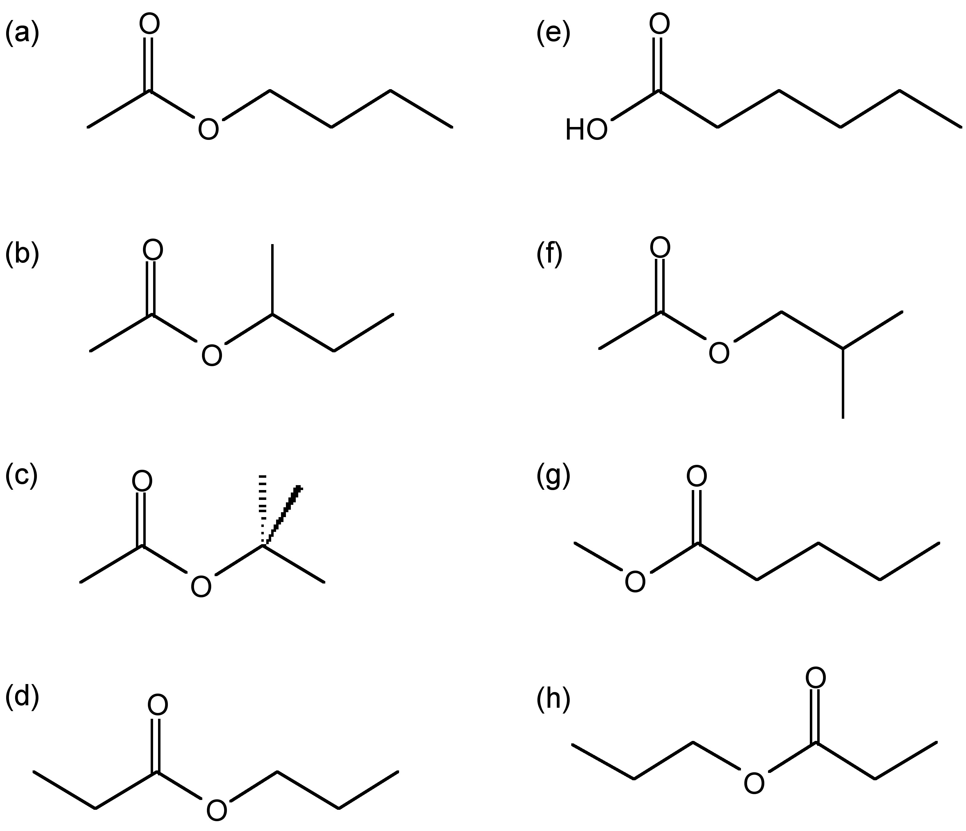
Structure of possible compounds with the molecular formula \(\ce{C6H12O2}\): (a) butylacetate, (b) sec-butyl acetate, (c) tert-butyl acetate, (d) ethyl butyrate, (e) haxanoic acid, (f) isobutyl acetate, (g) methyl pentanoate, and (h) propyl proponoate.

Exercise \(\PageIndex{3}\)

A 4.846 g sample containing carbon, hydrogen, and oxygen was burned in a combustion analysis apparatus; 4.843 g of \(\ce{H₂O}\) and 11.83 g of \(\ce{CO₂}\) were produced. Separately, the molar mass of the sample was found to be 144.22 g/mol. Determine the empirical formula, molecular formula, and identity of the sample.

Answer

The empirical formula is \(\ce{C₄H₈O}\), and the molecular formula is (\(\ce{C₄H₈O)₂}\) or \(\ce{C₈H₁₆O₂}\).

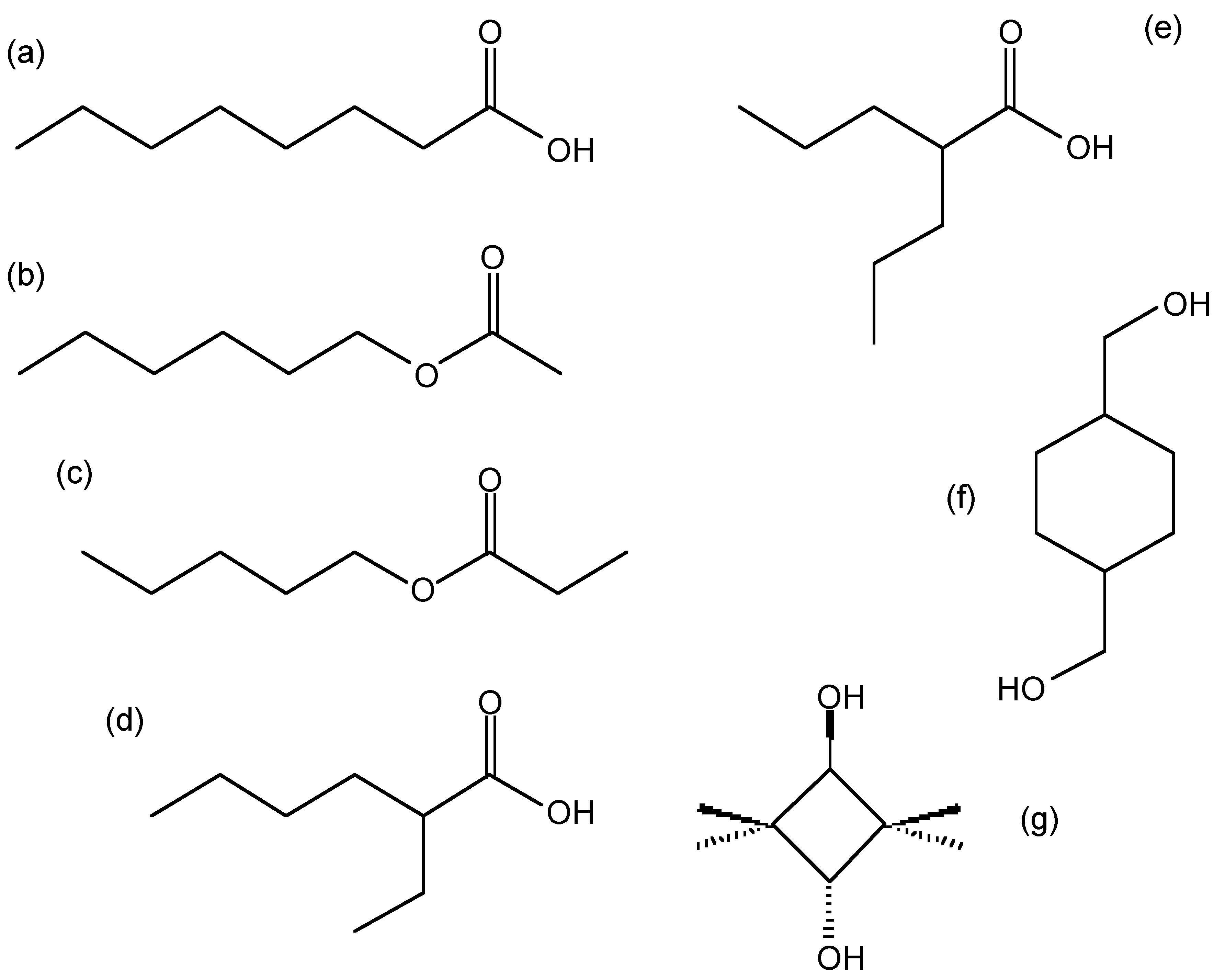
Structure of possible compounds with the molecular formula \(\ce{C8H16O2}\): (a) octanoic acid (caprylic acid), (b) hexyl acetate, (c) pentyl proponate, (d) 2-ethyl hexanoic acid, (e) valproic acid (VPA), (f) cyclohexanedimethanol (CHDM), and (g) 2,2,4,4-tetramethyl-1,3-cyclobutandiol (CBDO).

Binary compounds

By using combustion analysis, the chemical formula of a binary compound containing oxygen can also be determined. This is particularly helpful in the case of combustion of a metal which can result in potential oxides of multiple oxidation states.

Example \(\PageIndex{4}\):

A sample of iron weighing 1.7480 g is combusted in the presence of excess oxygen. A metal oxide (\(\ce{Fe_{x}O_{y})}\) is formed with a mass of 2.4982 g. Determine the chemical formula of the oxide product and the oxidation state of Fe.

Step 1: Subtract the mass of Fe from the mass of the oxide to determine the mass of oxygen in the product.

\[ 2.4982~\mathrm { g~Fe } _ { \mathrm { x } } \mathrm { O } _ { \mathrm { y } } - 1.7480~\mathrm { g~Fe } = 0.7502~\mathrm { g~O } \nonumber \]

Step 2: Using the molar masses of Fe and O, calculate the molar amounts of each element.

\[ 1.7480 \mathrm { g~Fe } \times \frac { 1 \text { mol Fe } } { 55.845 \text { g Fe } } = 0.031301 \text { mol Fe } \nonumber \]

\[ 0.7502~\text { g } \times \frac { 1 \text { mol O }} { 16.00~\text { g O} } = 0.04689~\text { mol O } \nonumber \]

Step 3: Divide the larger molar amount by the smaller molar amount. In some cases, the ratio is not made up of two integers. Convert the numerator of the ratio to an improper fraction and rewrite the ratio in whole numbers as shown.

\[ \frac { 0.031301~\text{ mol Fe } } { 0.04689~\mathrm { mol~O } } = \frac { 0.6675~\mathrm { mol~Fe } } { 1~\mathrm { mol~O } } = \frac{ \frac{2}{3} \mathrm { mol~Fe } } { 1~\mathrm { mol~O } } = \frac { 2~\mathrm { mol~Fe } } { 3~\mathrm { mol~O } } \nonumber \]

Therefore, the chemical formula of the oxide is \(\ce{Fe2O3}\), and Fe has a 3+ oxidation state.

Exercise \(\PageIndex{4}\)

A sample of copper weighing 7.295 g is combusted in the presence of excess oxygen. A metal oxide (\(\ce{Cu_{x}O_{y}}\)) is formed with a mass of 8.2131 g. Determine the chemical formula of the oxide product and the oxidation state of Cu.

Answer

The chemical formula is \(\ce{Cu2O}\), and Cu has a 1+ oxidation state..

Bibliography

• J. A. Dumas, Ann. Chem. Pharm., 1841, 38, 141.
• H. Goldwhite, J. Chem. Edu., 1978, 55, 366.
• A. Lavoisier, Traité Élémentaire de Chimie, 1789, 2, 493.
• J. Von Liebig, Annalen der Physik und Chemie, 1831, 21, 1.
• A. Linan and F. A. Williams, Fundamental Aspects of Combustion, Oxford University Press, New York (1993).
• J. M. McBride, "Combustion Analysis," Chemistry 125, Yale University.
• W. Prout, Philos. T. R. Soc. Lond., 1827, 117, 355.
• D. Shriver and P. Atkins, Inorganic Chemistry, 5^th Ed., W. H. Freeman and Co., New York (2009).
• W. Vining et. al., General Chemistry, 1^st Ed., Cengage, Brooks/Cole Cengage Learning, University of Massachusetts Amherst (2014).
• J. Warnatz, U. Maas, and R. W. Dibble, Combustion: Physical and Chemical Fundamentals, Modeling and Simulation, Experiments, Pollutant Formation, 3^rd Ed., Springer, Berlin (2001)