
2.1: Introduction
- Page ID
- 111361

\( \newcommand{\vecs}[1]{\overset { \scriptstyle \rightharpoonup} {\mathbf{#1}} } \)
\( \newcommand{\vecd}[1]{\overset{-\!-\!\rightharpoonup}{\vphantom{a}\smash {#1}}} \)
\( \newcommand{\id}{\mathrm{id}}\) \( \newcommand{\Span}{\mathrm{span}}\)
( \newcommand{\kernel}{\mathrm{null}\,}\) \( \newcommand{\range}{\mathrm{range}\,}\)
\( \newcommand{\RealPart}{\mathrm{Re}}\) \( \newcommand{\ImaginaryPart}{\mathrm{Im}}\)
\( \newcommand{\Argument}{\mathrm{Arg}}\) \( \newcommand{\norm}[1]{\| #1 \|}\)
\( \newcommand{\inner}[2]{\langle #1, #2 \rangle}\)
\( \newcommand{\Span}{\mathrm{span}}\)
\( \newcommand{\id}{\mathrm{id}}\)
\( \newcommand{\Span}{\mathrm{span}}\)
\( \newcommand{\kernel}{\mathrm{null}\,}\)
\( \newcommand{\range}{\mathrm{range}\,}\)
\( \newcommand{\RealPart}{\mathrm{Re}}\)
\( \newcommand{\ImaginaryPart}{\mathrm{Im}}\)
\( \newcommand{\Argument}{\mathrm{Arg}}\)
\( \newcommand{\norm}[1]{\| #1 \|}\)
\( \newcommand{\inner}[2]{\langle #1, #2 \rangle}\)
\( \newcommand{\Span}{\mathrm{span}}\) \( \newcommand{\AA}{\unicode[.8,0]{x212B}}\)
\( \newcommand{\vectorA}[1]{\vec{#1}} % arrow\)
\( \newcommand{\vectorAt}[1]{\vec{\text{#1}}} % arrow\)
\( \newcommand{\vectorB}[1]{\overset { \scriptstyle \rightharpoonup} {\mathbf{#1}} } \)
\( \newcommand{\vectorC}[1]{\textbf{#1}} \)
\( \newcommand{\vectorD}[1]{\overrightarrow{#1}} \)
\( \newcommand{\vectorDt}[1]{\overrightarrow{\text{#1}}} \)
\( \newcommand{\vectE}[1]{\overset{-\!-\!\rightharpoonup}{\vphantom{a}\smash{\mathbf {#1}}}} \)
\( \newcommand{\vecs}[1]{\overset { \scriptstyle \rightharpoonup} {\mathbf{#1}} } \)
\( \newcommand{\vecd}[1]{\overset{-\!-\!\rightharpoonup}{\vphantom{a}\smash {#1}}} \)
\(\newcommand{\avec}{\mathbf a}\) \(\newcommand{\bvec}{\mathbf b}\) \(\newcommand{\cvec}{\mathbf c}\) \(\newcommand{\dvec}{\mathbf d}\) \(\newcommand{\dtil}{\widetilde{\mathbf d}}\) \(\newcommand{\evec}{\mathbf e}\) \(\newcommand{\fvec}{\mathbf f}\) \(\newcommand{\nvec}{\mathbf n}\) \(\newcommand{\pvec}{\mathbf p}\) \(\newcommand{\qvec}{\mathbf q}\) \(\newcommand{\svec}{\mathbf s}\) \(\newcommand{\tvec}{\mathbf t}\) \(\newcommand{\uvec}{\mathbf u}\) \(\newcommand{\vvec}{\mathbf v}\) \(\newcommand{\wvec}{\mathbf w}\) \(\newcommand{\xvec}{\mathbf x}\) \(\newcommand{\yvec}{\mathbf y}\) \(\newcommand{\zvec}{\mathbf z}\) \(\newcommand{\rvec}{\mathbf r}\) \(\newcommand{\mvec}{\mathbf m}\) \(\newcommand{\zerovec}{\mathbf 0}\) \(\newcommand{\onevec}{\mathbf 1}\) \(\newcommand{\real}{\mathbb R}\) \(\newcommand{\twovec}[2]{\left[\begin{array}{r}#1 \\ #2 \end{array}\right]}\) \(\newcommand{\ctwovec}[2]{\left[\begin{array}{c}#1 \\ #2 \end{array}\right]}\) \(\newcommand{\threevec}[3]{\left[\begin{array}{r}#1 \\ #2 \\ #3 \end{array}\right]}\) \(\newcommand{\cthreevec}[3]{\left[\begin{array}{c}#1 \\ #2 \\ #3 \end{array}\right]}\) \(\newcommand{\fourvec}[4]{\left[\begin{array}{r}#1 \\ #2 \\ #3 \\ #4 \end{array}\right]}\) \(\newcommand{\cfourvec}[4]{\left[\begin{array}{c}#1 \\ #2 \\ #3 \\ #4 \end{array}\right]}\) \(\newcommand{\fivevec}[5]{\left[\begin{array}{r}#1 \\ #2 \\ #3 \\ #4 \\ #5 \\ \end{array}\right]}\) \(\newcommand{\cfivevec}[5]{\left[\begin{array}{c}#1 \\ #2 \\ #3 \\ #4 \\ #5 \\ \end{array}\right]}\) \(\newcommand{\mattwo}[4]{\left[\begin{array}{rr}#1 \amp #2 \\ #3 \amp #4 \\ \end{array}\right]}\) \(\newcommand{\laspan}[1]{\text{Span}\{#1\}}\) \(\newcommand{\bcal}{\cal B}\) \(\newcommand{\ccal}{\cal C}\) \(\newcommand{\scal}{\cal S}\) \(\newcommand{\wcal}{\cal W}\) \(\newcommand{\ecal}{\cal E}\) \(\newcommand{\coords}[2]{\left\{#1\right\}_{#2}}\) \(\newcommand{\gray}[1]{\color{gray}{#1}}\) \(\newcommand{\lgray}[1]{\color{lightgray}{#1}}\) \(\newcommand{\rank}{\operatorname{rank}}\) \(\newcommand{\row}{\text{Row}}\) \(\newcommand{\col}{\text{Col}}\) \(\renewcommand{\row}{\text{Row}}\) \(\newcommand{\nul}{\text{Nul}}\) \(\newcommand{\var}{\text{Var}}\) \(\newcommand{\corr}{\text{corr}}\) \(\newcommand{\len}[1]{\left|#1\right|}\) \(\newcommand{\bbar}{\overline{\bvec}}\) \(\newcommand{\bhat}{\widehat{\bvec}}\) \(\newcommand{\bperp}{\bvec^\perp}\) \(\newcommand{\xhat}{\widehat{\xvec}}\) \(\newcommand{\vhat}{\widehat{\vvec}}\) \(\newcommand{\uhat}{\widehat{\uvec}}\) \(\newcommand{\what}{\widehat{\wvec}}\) \(\newcommand{\Sighat}{\widehat{\Sigma}}\) \(\newcommand{\lt}{<}\) \(\newcommand{\gt}{>}\) \(\newcommand{\amp}{&}\) \(\definecolor{fillinmathshade}{gray}{0.9}\)Compare and contrast the absorption of ultraviolet (UV) and visible (VIS) radiation by an atomic substance (something like helium) with that of a molecular substance (something like ethylene).
Do you expect different absorption peaks or bands from an atomic or molecular substance to have different intensities? If so, what does this say about the transitions?
UV/VIS radiation has the proper energy to excite valence electrons of chemical species and cause electronic transitions.
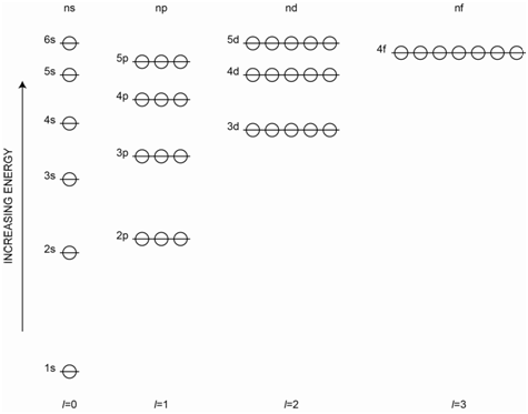
For atoms, the only process we need to think about is the excitation of electrons, (i.e., electronic transitions), from one atomic orbital to another. Since the atomic orbitals have discrete or specific energies, transitions among them have discrete or specific energies. Therefore, atomic absorption spectra consist of a series of “lines” at the wavelengths of radiation (or frequency of radiation) that correspond in energy to each allowable electronic transition. The diagram in Figure \(\PageIndex{1}\) represents the energy level diagram of any multielectron atom.
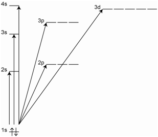
The different lines in the spectrum will have different intensities. As we have already discussed, different transitions have different probabilities or different molar absorptivities, which accounts for the different intensities. The process of absorption for helium is shown in Figure \(\PageIndex{2}\) in which one electron is excited to a higher energy orbital. Several possible absorption transitions are illustrated in the diagram.
The illustration in Figure \(\PageIndex{3}\) represents the atomic emission spectrum of helium and clearly shows the “line” nature of an atomic spectrum.

For molecules, there are two other important processes to consider besides the excitation of electrons from one molecular orbital to another. The first is that molecules vibrate. Molecular vibrations or vibrational transitions occur in the infrared portion of the spectrum and are therefore lower in energy than electronic transitions. The second is that molecules can rotate. Molecular rotations or rotational transitions occur in the microwave portion of the spectrum and are therefore lower in energy than electronic and vibrational transitions. The diagram in Figure \(\PageIndex{4}\) represents the energy level diagram for a molecule. The arrows in the diagram represent possible transitions from the ground to excited states.
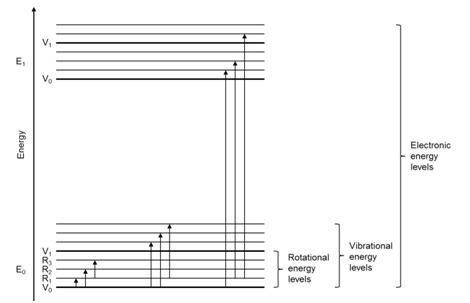
Note that the vibrational and rotational energy levels in a molecule are superimposed over the electronic transitions. An important question to consider is whether an electron in the ground state (lowest energy electronic, vibrational and rotational state) can only be excited to the first excited electronic state (no extra vibrational or rotational energy), or whether it can also be excited to vibrationally and/or rotationally excited states in the first excited electronic state. It turns out that molecules can be excited to vibrationally and/or rotationally excited levels of the first excited electronic state, as shown by arrows in Figure \(\PageIndex{4}\). Molecules can also be excited to the second and higher excited electronic states. Therefore, we can speak of a molecule as existing in the second excited rotational state of the third excited vibrational state of the first excited electronic state.
One consequence in the comparison of atomic and molecule absorption spectra is that molecular absorption spectra ought to have many more transitions or lines in them than atomic spectra because of all the vibrational and rotational excited states that exist.
Compare a molecular absorption spectrum of a dilute species dissolved in a solvent at room temperature versus the same sample at 10K.
The difference to consider here is that the sample at 10K will be frozen into a solid whereas the sample at room temperature will be a liquid. In the liquid state, the solute and solvent molecules move about via diffusion and undergo frequent collisions with each other. In the solid state, collisions are reduced considerably.
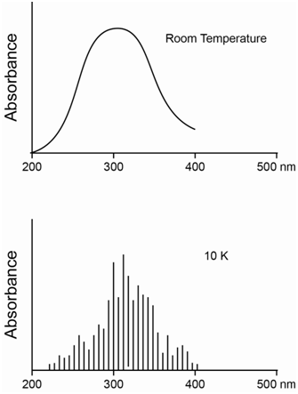
What is the effect of collisions of solvent and solute molecules? Collisions between molecules cause distortions of the electrons. Since molecules in a mixture move with a distribution of different speeds, the collisions occur with different degrees of distortion of the electrons. Since the energy of electrons depends on their locations in space, distortion of the electrons causes slight changes in the energy of the electrons. Slight changes in the energy of an electron means there will be a slight change in the energy of its transition to a higher energy state. The net effect of collisions is to cause a broadening of the lines in the spectrum. The spectrum at room temperature will show significant collisional broadening whereas the spectrum at 10K will have minimal collisional broadening. The collisional broadening at room temperature in a solvent such as water is significant enough to cause a blurring together of the energy differences between the different rotational and vibrational states, such that the spectrum consists of broad absorption bands instead of discrete lines. By contrast, the spectrum at 10K will consist of numerous discrete lines that distinguish between the different rotationally and vibrationally excited levels of the excited electronic states. The diagrams in Figure \(\PageIndex{5}\) show the difference between the spectrum at room temperature and 10K, although the one at 10K does not contain nearly the number of lines that would be observed in the actual spectrum.
Are there any other general processes that contribute to broadening in an absorption spectrum?
The other general contribution to broadening comes from something known as the Doppler Effect. The Doppler Effect occurs because the species absorbing or emitting radiation is moving relative to the detector. Perhaps the easiest way to think about this is to consider a species moving away from the detector that emits a specific frequency of radiation heading toward the detector. The frequency of radiation corresponds to that of the energy of the transition, so the emitted radiation has a specific, fixed frequency. The picture in Figure \(\PageIndex{6}\) shows two species emitting waves of radiation toward a detector. It is worth focusing on the highest amplitude portion of each wave. Also, in Figure \(\PageIndex{6}\), assume that the detector is on the right side of the diagram and the right side of the two emitting spheres. The emission process to produce the wave of radiation requires some finite amount of time. If the species is moving away from the detector, even though the frequency is fixed, to the detector it will appear as if each of the highest amplitude regions of the wave is lagging behind where they would be if the species is stationary (see the upper sphere in Figure \(\PageIndex{6}\)). The result is that the wavelength of the radiation appears longer, meaning that the frequency appears lower. For visible radiation, we say that the radiation from the emitting species is red-shifted. The lower sphere in Figure \(\PageIndex{6}\) is moving towards the detector. Now the highest amplitude regions of the wave are appearing at the detector faster than expected. This radiation is blue-shifted. In a solution, different species are moving in different directions relative to the detector. Some exhibit no Doppler shift. Others would be blue-shifted whereas others would be red-shifted and the degree of red- and blue-shift varies among different species. The net effect would be that the emission peak is broadened. The same process occurs with the absorption of radiation as well.
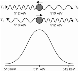
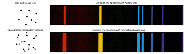
The emission spectrum in Figure \(\PageIndex{7}\) represents the Doppler broadening that would occur for a gas phase atomic species where the atoms are not moving (top) and then moving with random motion (bottom).
A practical application of the Doppler Effect is the measurement of the distance of galaxies from the earth. The universe is expanding away from a central point. Hubble’s Law and the Hubble effect is an observation that the further a galaxy is from the center of the universe, the faster it moves. There is also a precise formula that predicts the speed of movement relative to the distance from the center of the universe. Galaxies further from the center of the universe therefore show a larger red shift in their radiation due to the Doppler Effect than galaxies closer to the center of the universe. Measurements of the red-shift are used to determine the placement of galaxies in the universe.