34.1: Overview

What Do We Mean By a Particle?

Particles come in many forms. Some are very small, such as nanoparticles with dimensions of 1-100 nm and that might consist of just a few hundred atoms, and some are much larger, as in the beads of ion-exchange resin shown in Figure \(\PageIndex{1}\), which range in size from approximately 300 µm to 850 µm. Or, consider soils, which generally are subdivided into four types of particles: clay, which has particles with diameters smaller than 2 µm, silt, which has particle with diameters that range from 2 µm to 50 µm, sand, which has particle with diameters from 50 µm to 2000 µm, and gravel, which has particles with diameters larger than 2000 µm in size.

Figure \(\PageIndex{1}\): Example of an ion-exchange resin. The individual beads seen here range in size from approximately 300 µm to 850 µm in diameter.

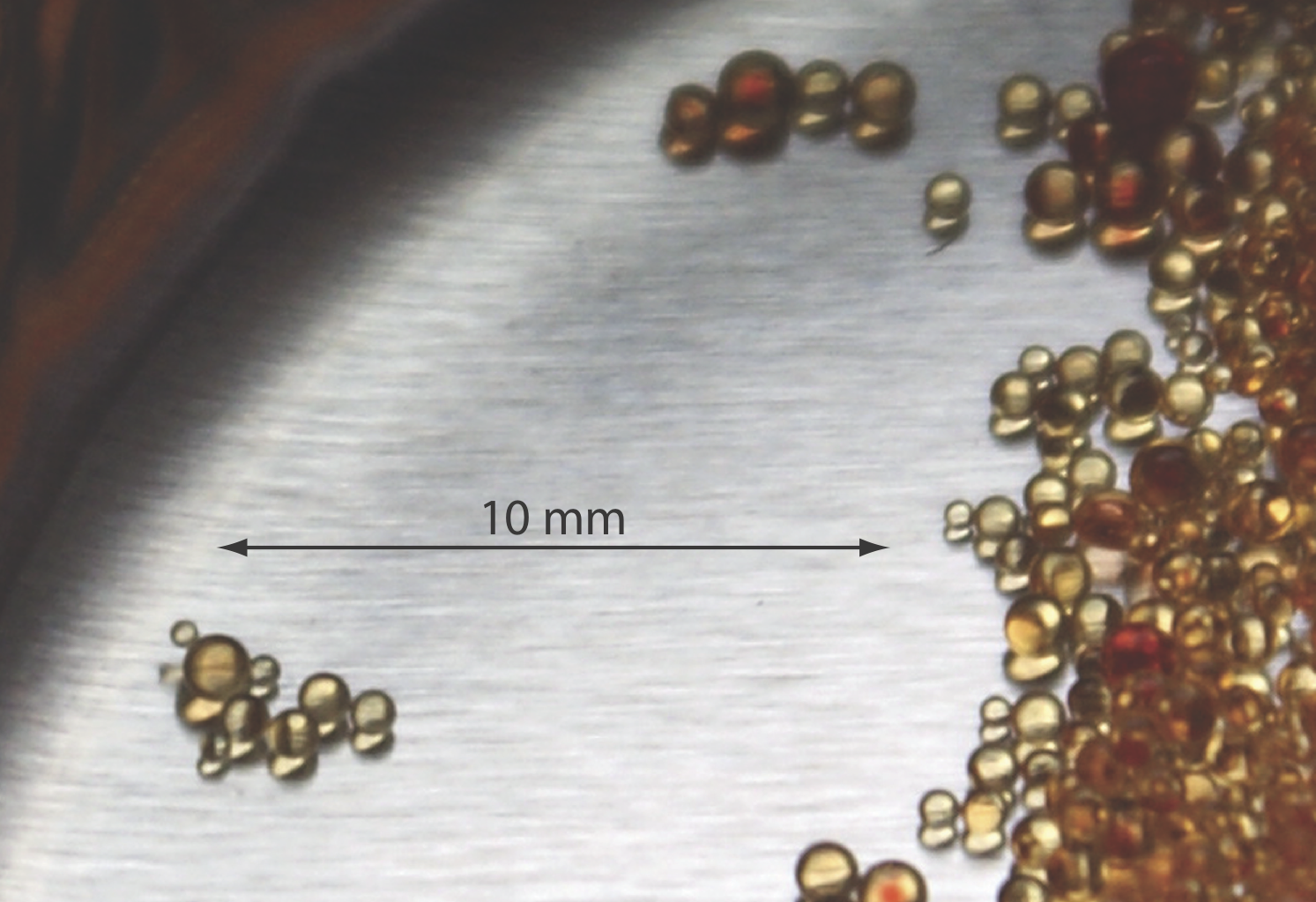
We often hold as an image that particles are spherical in shape, which means we can characterize them by reporting a single number: the particle's diameter. Many particulate materials, however, are not uniform in shape. Although many of the resin beads in Figure \(\PageIndex{1}\) appear spherical—the largest bead in the small cluster at the left certainly looks spherical—others of the resin beads are distorted in shape, often appearing somewhat flattened. Still, it is not unusual to treat particles as if they are spheres. There are a number of reasons for this. If the method we use to determine size is not based on a static image (as is the case in Figure \(\PageIndex{1}\)), but on a suspension of particles that are rotating rapidly on the timescale of our measurement, then the particle's shape averages out to a sphere even if the particle itself is not a sphere. The size we report, in this case, is called an equivalent spherical diameter (ESD), which may vary from method-to-method.

How do We Report Particle Size?

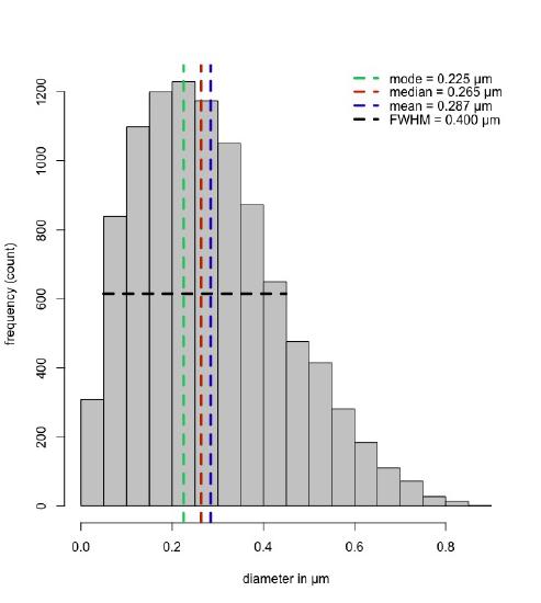
Suppose we use a method to determine the size of 10000 particles. A simple way to display the data is to use a histogram that reports the frequency of particles in different size ranges, as we see in Figure \(\PageIndex{2}\). We can characterize this distribution by reporting one or more measures of its central tendency and a measure of its spread.

Typical measures of central tendency are the mode, which is the most common result, the median, which is the result that falls exactly in the middle of all recorded values, and the mean, which is the numerical average. For the data in Figure \(\PageIndex{2}\), the mode is 0.255 µm (the center of the bin that begins at 0.200 µm and ends at 0.250 µm), the median is 0.265 µm, and the mean is 0.287 µm. If the distribution was symmetrical, then the mode, median, and mean would be identical; here, the distribution has a long tail to the right, which increases the mean relative to the median, and increases the mean and the median relative to the mode.

A common way to report the spread is to use the width of the distribution at a frequency that is half of the maximum frequency; this is called the full-width-at-half-maximum (FWHM). For the data in Figure \(\PageIndex{2}\), the maximum frequency is 1230 counts. The FWHM is at a frequency of 615 and runs from a diameter of 0.050 µm to 0.450 µm, or FWHM = 0.450 – 0.050 = 0.400 µm.

Figure \(\PageIndex{2}\): Histogram that shows the distribution of particle sizes for a sample consisting of 10000 particles. Each bin has a size of 0.05 µm. The mode, median, and mean diameters are shown by the vertical dashed lines. The horizontal dashed line show the data's full-width-at-half-maximum.

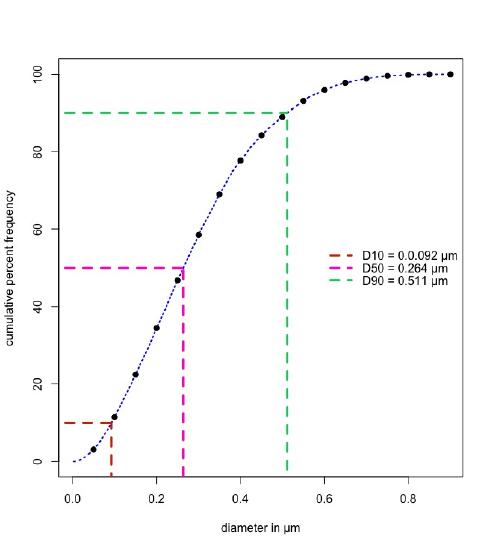
Another way to characterize the distribution of particle sizes is to plot the cumulative frequency (as a percent) as a function of the diameter of the particles. Figure \(\PageIndex{3}\) shows this for the data in Figure \(\PageIndex{2}\) using both the binned data for the histogram (shown as the circular black points), and using all of the underlying data (shown as the dashed blue line). The red, purple, and green lines show the particle diameters that include 10% (D10), 50% (D50), and 90% (D90) of all particles. The value of 0.264 µm indicates that half of the particles have diameters less than 0.264 µm and that half have diameters greater than 0.264 µm. One measure of the distribution's relative width is the span, which is defined as

\[\text{span} = \frac{\text{D90} - \text{D10}}{\text{D50}} = \frac{0.511 - 0.093}{0.264} = 1.59 \nonumber \]

Figure \(\PageIndex{3}\): The cumulative distribution of the data from Figure \(\PageIndex{2}\). The dashed lines show the D10, D50, and D90 values.

How Can We Measure Particle Size?

There are a variety of methods that we can use to determine the distribution in the sizes of a particulate material, more than we can cover in a single chapter. Instead, we will consider four common methods: sieving, sedimentation, imaging, and light scattering. When choosing a method, the size and form of the particles are important factors. Sieving, for example, is a practical choice when working with solid particulates that have diameters as small as 20 µm and as large as 125 mm (Note the change from µm to mm!). Sedimentation is useful for particles with diameters of 1 µm, which we can extend to diameters as small as 1 nm by using a centrifuge. Image analysis is useful for particles between 0.5 µm and 1500 µm. Finally, light scattering is useful for particles as small as 0.8 nm.