
25.7: Applications of Voltammetry
- Page ID
- 335305

\( \newcommand{\vecs}[1]{\overset { \scriptstyle \rightharpoonup} {\mathbf{#1}} } \)
\( \newcommand{\vecd}[1]{\overset{-\!-\!\rightharpoonup}{\vphantom{a}\smash {#1}}} \)
\( \newcommand{\dsum}{\displaystyle\sum\limits} \)
\( \newcommand{\dint}{\displaystyle\int\limits} \)
\( \newcommand{\dlim}{\displaystyle\lim\limits} \)
\( \newcommand{\id}{\mathrm{id}}\) \( \newcommand{\Span}{\mathrm{span}}\)
( \newcommand{\kernel}{\mathrm{null}\,}\) \( \newcommand{\range}{\mathrm{range}\,}\)
\( \newcommand{\RealPart}{\mathrm{Re}}\) \( \newcommand{\ImaginaryPart}{\mathrm{Im}}\)
\( \newcommand{\Argument}{\mathrm{Arg}}\) \( \newcommand{\norm}[1]{\| #1 \|}\)
\( \newcommand{\inner}[2]{\langle #1, #2 \rangle}\)
\( \newcommand{\Span}{\mathrm{span}}\)
\( \newcommand{\id}{\mathrm{id}}\)
\( \newcommand{\Span}{\mathrm{span}}\)
\( \newcommand{\kernel}{\mathrm{null}\,}\)
\( \newcommand{\range}{\mathrm{range}\,}\)
\( \newcommand{\RealPart}{\mathrm{Re}}\)
\( \newcommand{\ImaginaryPart}{\mathrm{Im}}\)
\( \newcommand{\Argument}{\mathrm{Arg}}\)
\( \newcommand{\norm}[1]{\| #1 \|}\)
\( \newcommand{\inner}[2]{\langle #1, #2 \rangle}\)
\( \newcommand{\Span}{\mathrm{span}}\) \( \newcommand{\AA}{\unicode[.8,0]{x212B}}\)
\( \newcommand{\vectorA}[1]{\vec{#1}} % arrow\)
\( \newcommand{\vectorAt}[1]{\vec{\text{#1}}} % arrow\)
\( \newcommand{\vectorB}[1]{\overset { \scriptstyle \rightharpoonup} {\mathbf{#1}} } \)
\( \newcommand{\vectorC}[1]{\textbf{#1}} \)
\( \newcommand{\vectorD}[1]{\overrightarrow{#1}} \)
\( \newcommand{\vectorDt}[1]{\overrightarrow{\text{#1}}} \)
\( \newcommand{\vectE}[1]{\overset{-\!-\!\rightharpoonup}{\vphantom{a}\smash{\mathbf {#1}}}} \)
\( \newcommand{\vecs}[1]{\overset { \scriptstyle \rightharpoonup} {\mathbf{#1}} } \)
\(\newcommand{\longvect}{\overrightarrow}\)
\( \newcommand{\vecd}[1]{\overset{-\!-\!\rightharpoonup}{\vphantom{a}\smash {#1}}} \)
\(\newcommand{\avec}{\mathbf a}\) \(\newcommand{\bvec}{\mathbf b}\) \(\newcommand{\cvec}{\mathbf c}\) \(\newcommand{\dvec}{\mathbf d}\) \(\newcommand{\dtil}{\widetilde{\mathbf d}}\) \(\newcommand{\evec}{\mathbf e}\) \(\newcommand{\fvec}{\mathbf f}\) \(\newcommand{\nvec}{\mathbf n}\) \(\newcommand{\pvec}{\mathbf p}\) \(\newcommand{\qvec}{\mathbf q}\) \(\newcommand{\svec}{\mathbf s}\) \(\newcommand{\tvec}{\mathbf t}\) \(\newcommand{\uvec}{\mathbf u}\) \(\newcommand{\vvec}{\mathbf v}\) \(\newcommand{\wvec}{\mathbf w}\) \(\newcommand{\xvec}{\mathbf x}\) \(\newcommand{\yvec}{\mathbf y}\) \(\newcommand{\zvec}{\mathbf z}\) \(\newcommand{\rvec}{\mathbf r}\) \(\newcommand{\mvec}{\mathbf m}\) \(\newcommand{\zerovec}{\mathbf 0}\) \(\newcommand{\onevec}{\mathbf 1}\) \(\newcommand{\real}{\mathbb R}\) \(\newcommand{\twovec}[2]{\left[\begin{array}{r}#1 \\ #2 \end{array}\right]}\) \(\newcommand{\ctwovec}[2]{\left[\begin{array}{c}#1 \\ #2 \end{array}\right]}\) \(\newcommand{\threevec}[3]{\left[\begin{array}{r}#1 \\ #2 \\ #3 \end{array}\right]}\) \(\newcommand{\cthreevec}[3]{\left[\begin{array}{c}#1 \\ #2 \\ #3 \end{array}\right]}\) \(\newcommand{\fourvec}[4]{\left[\begin{array}{r}#1 \\ #2 \\ #3 \\ #4 \end{array}\right]}\) \(\newcommand{\cfourvec}[4]{\left[\begin{array}{c}#1 \\ #2 \\ #3 \\ #4 \end{array}\right]}\) \(\newcommand{\fivevec}[5]{\left[\begin{array}{r}#1 \\ #2 \\ #3 \\ #4 \\ #5 \\ \end{array}\right]}\) \(\newcommand{\cfivevec}[5]{\left[\begin{array}{c}#1 \\ #2 \\ #3 \\ #4 \\ #5 \\ \end{array}\right]}\) \(\newcommand{\mattwo}[4]{\left[\begin{array}{rr}#1 \amp #2 \\ #3 \amp #4 \\ \end{array}\right]}\) \(\newcommand{\laspan}[1]{\text{Span}\{#1\}}\) \(\newcommand{\bcal}{\cal B}\) \(\newcommand{\ccal}{\cal C}\) \(\newcommand{\scal}{\cal S}\) \(\newcommand{\wcal}{\cal W}\) \(\newcommand{\ecal}{\cal E}\) \(\newcommand{\coords}[2]{\left\{#1\right\}_{#2}}\) \(\newcommand{\gray}[1]{\color{gray}{#1}}\) \(\newcommand{\lgray}[1]{\color{lightgray}{#1}}\) \(\newcommand{\rank}{\operatorname{rank}}\) \(\newcommand{\row}{\text{Row}}\) \(\newcommand{\col}{\text{Col}}\) \(\renewcommand{\row}{\text{Row}}\) \(\newcommand{\nul}{\text{Nul}}\) \(\newcommand{\var}{\text{Var}}\) \(\newcommand{\corr}{\text{corr}}\) \(\newcommand{\len}[1]{\left|#1\right|}\) \(\newcommand{\bbar}{\overline{\bvec}}\) \(\newcommand{\bhat}{\widehat{\bvec}}\) \(\newcommand{\bperp}{\bvec^\perp}\) \(\newcommand{\xhat}{\widehat{\xvec}}\) \(\newcommand{\vhat}{\widehat{\vvec}}\) \(\newcommand{\uhat}{\widehat{\uvec}}\) \(\newcommand{\what}{\widehat{\wvec}}\) \(\newcommand{\Sighat}{\widehat{\Sigma}}\) \(\newcommand{\lt}{<}\) \(\newcommand{\gt}{>}\) \(\newcommand{\amp}{&}\) \(\definecolor{fillinmathshade}{gray}{0.9}\)Voltammetry finds use for both quantitative analyses and characterization analyses. Examples of each are highlighted in this section.
Quantitative Applications
Voltammetry has been used for the quantitative analysis of a wide variety of samples, including environmental samples, clinical samples, pharmaceutical formulations, steels, gasoline, and oil.
Selecting the Voltammetric Technique
The choice of which voltammetric technique to use depends on the sample’s characteristics, including the analyte’s expected concentration and the sample’s location. For example, amperometry is ideally suited for detecting analytes in flow systems, including the in vivo analysis of a patient’s blood or as a selective sensor for the rapid analysis of a single analyte. The portability of amperometric sensors, which are similar to potentiometric sensors, also make them ideal for field studies. Although cyclic voltammetry is used to determine an analyte’s concentration, other methods described in this chapter are better suited for quantitative work.
Pulse polarography and stripping voltammetry frequently are interchangeable. The choice of which technique to use often depends on the analyte’s concentration and the desired accuracy and precision. Detection limits for normal pulse polarography generally are on the order of 10–6 M to 10–7 M, and those for differential pulse polarography, staircase, and square wave polarography are between 10–7 M and 10–9 M. Because we concentrate the analyte in stripping voltammetry, the detection limit for many analytes is as little as 10–10 M to 10–12 M. On the other hand, the current in stripping voltammetry is much more sensitive than pulse polarography to changes in experimental conditions, which may lead to poorer precision and accuracy. We also can use pulse polarography to analyze a wider range of inorganic and organic analytes because there is no need to first deposit the analyte at the electrode surface.
Stripping voltammetry also suffers from occasional interferences when two metals, such as Cu and Zn, combine to form an intermetallic compound in the mercury amalgam. The deposition potential for Zn is sufficiently negative that any Cu2+ in the sample also deposits into the mercury drop or film, leading to the formation of intermetallic compounds such as CuZn and CuZn2. During the stripping step, zinc in the intermetallic compounds strips at potentials near that of copper, decreasing the current for zinc at its usual potential and increasing the apparent current for copper. It is possible to overcome this problem by adding an element that forms a stronger intermetallic compound with the interfering metal. Thus, adding Ga3+ minimizes the interference of Cu when analyzing for Zn by forming an intermetallic compound of Cu and Ga.
Correcting for the Residual Current
In any quantitative analysis we must correct the analyte’s signal for signals that arise from other sources. The total current, itot, in voltammetry consists of two parts: the current from the analyte’s oxidation or reduction, iA, and a background or residual current, ir.
\[i_{t o t}=i_{A}+i_{r} \label{app1} \]
The residual current, in turn, has two sources. One source is a faradaic current from the oxidation or reduction of trace interferents in the sample, iint. The other source is the charging current, ich, that accompanies a change in the working electrode’s potential.
\[i_{r}=i_{\mathrm{int}}+i_{c h} \label{app2} \]
We can minimize the faradaic current due to impurities by carefully preparing the sample. For example, one important impurity is dissolved O2, which undergoes a two-step reduction: first to H2O2 at a potential of –0.1 V versus the SCE, and then to H2O at a potential of –0.9 V versus the SCE. Removing dissolved O2 by bubbling an inert gas such as N2 through the sample eliminates this interference. After removing the dissolved O2, maintaining a blanket of N2 over the top of the solution prevents O2 from reentering the solution.
There are two methods to compensate for the residual current. One method is to measure the total current at potentials where the analyte’s faradaic current is zero and extrapolate it to other potentials. This is the method shown in Figure 25.3.7. One advantage of extrapolating is that we do not need to acquire additional data. An important disadvantage is that an extrapolation assumes that any change in the residual current with potential is predictable, which may not be the case. A second, and more rigorous approach, is to obtain a voltammogram for an appropriate blank. The blank’s residual current is then subtracted from the sample’s total current.
Analysis for Single Components
The analysis of a sample with a single analyte is straightforward using any of the standardization methods discussed in Chapter 1.
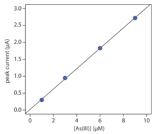
The concentration of As(III) in water is determined by differential pulse polarography in 1 M HCl. The initial potential is set to –0.1 V versus the SCE and is scanned toward more negative potentials at a rate of 5 mV/s. Reduction of As(III) to As(0) occurs at a potential of approximately –0.44 V versus the SCE. The peak currents for a set of standard solutions, corrected for the residual current, are shown in the following table.
| [As(III)] (µM) | ip (µM) |
|---|---|
| 1.00 | 0.298 |
| 3.00 | 0.947 |
| 6.00 | 1.83 |
| 9.00 | 2.72 |
What is the concentration of As(III) in a sample of water if its peak current is 1.37 μA?
Solution
Linear regression gives the calibration curve shown in Figure \(\PageIndex{1}\), with an equation of
\[i_{p}=0.0176+3.01 \times[\mathrm{As}(\mathrm{III})] \nonumber \]
Substituting the sample’s peak current into the regression equation gives the concentration of As(III) as 4.49 μM.
Multicomponent Analysis
Voltammetry is a particularly attractive technique for the analysis of samples that contain two or more analytes. Provided that the analytes behave independently, the voltammogram of a multicomponent mixture is a summation of each analyte’s individual voltammograms. As shown in Figure \(\PageIndex{2}\), if the separation between the half-wave potentials or between the peak potentials is sufficient, we can determine the presence of each analyte as if it is the only analyte in the sample. The minimum separation between the half-wave potentials or peak potentials for two analytes depends on several factors, including the type of electrode and the potential-excitation signal. For normal polarography the separation is at least ±0.2–0.3 V, and differential pulse voltammetry requires a minimum separation of ±0.04–0.05 V.
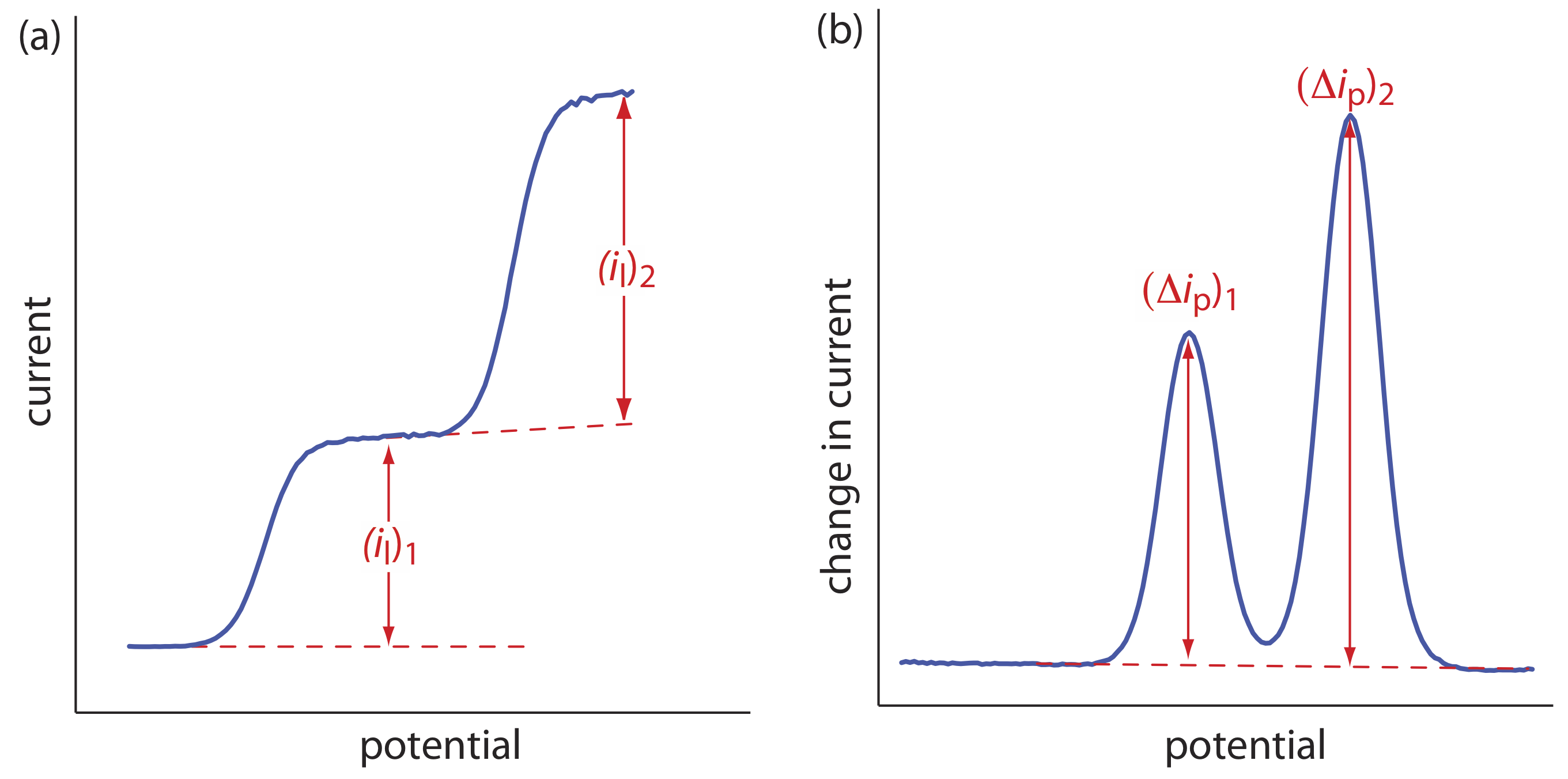
If the voltammograms for two analytes are not sufficiently separated, a simultaneous analysis may be possible. An example of this approach is outlined the following example.
The differential pulse polarographic analysis of a mixture of indium and cadmium in 0.1 M HCl is complicated by the overlap of their respective voltammograms [Lanza P. J. Chem. Educ. 1990, 67, 704–705]. The peak potential for indium is at –0.557 V and that for cadmium is at –0.597 V. When a 0.800-ppm indium standard is analyzed, \(\Delta i_p\) (in arbitrary units) is 200.5 at –0.557 V and 87.5 at –0.597 V relative to a saturated Ag/AgCl reference electorde. A standard solution of 0.793 ppm cadmium has a \(\Delta i_p\) of 58.5 at –0.557 V and 128.5 at –0.597 V. What is the concentration of indium and cadmium in a sample if \(\Delta i_p\) is 167.0 at a potential of –0.557 V and 99.5 at a potential of –0.597V.
Solution
The change in current, \(\Delta i_p\), in differential pulse polarography is a linear function of the analyte’s concentration
\[\Delta i_{p}=k_{A} C_{A} \nonumber \]
where kA is a constant that depends on the analyte and the applied potential, and CA is the analyte’s concentration. To determine the concentrations of indium and cadmium in the sample we must first find the value of kA for each analyte at each potential. For simplicity we will identify the potential of –0.557 V as E1, and that for –0.597 V as E2. The values of kA are
\[\begin{aligned} k_{\mathrm{In}, E_{1}} &=\frac{200.5}{0.800 \ \mathrm{ppm}}=250.6 \ \mathrm{ppm}^{-1} \\ k_{\mathrm{In}, E_{2}} &=\frac{87.5}{0.800 \ \mathrm{ppm}}=109.4 \ \mathrm{ppm}^{-1} \\ k_{\mathrm{Cd} E_{1}} &=\frac{58.5}{0.793 \ \mathrm{ppm}}=73.8 \ \mathrm{ppm}^{-1} \\ k_{\mathrm{Cd} E_{2}} &=\frac{128.5}{0.793 \ \mathrm{ppm}}=162.0 \ \mathrm{ppm}^{-1} \end{aligned} \nonumber \]
Next, we write simultaneous equations for the current at the two potentials.
\[\begin{array}{l}{\Delta i_{E_{1}}=167.0=250.6 \ \mathrm{ppm}^{-1} \times C_{\mathrm{In}}+73.8 \ \mathrm{ppm}^{-1} \times C_{\mathrm{Cd}}} \\ {\triangle i_{E_{2}}=99.5=109.4 \ \mathrm{ppm}^{-1} \times C_{\mathrm{In}}+162.0 \ \mathrm{ppm}^{-1} \times C_{\mathrm{Cd}}}\end{array} \nonumber \]
Solving the simultaneous equations, which is left as an exercise, gives the concentration of indium as 0.606 ppm and the concentration of cadmium as 0.205 ppm.
Environmental Samples
Voltammetry is one of several important analytical techniques for the analysis of trace metals in environmental samples, including groundwater, lakes, rivers and streams, seawater, rain, and snow. Detection limits at the parts-per-billion level are routine for many trace metals using differential pulse polarography, with anodic stripping voltammetry providing parts-per-trillion detection limits for some trace metals.
One interesting environmental application of anodic stripping voltammetry is the determination of a trace metal’s chemical form within a water sample. Speciation is important because a trace metal’s bioavailability, toxicity, and ease of transport through the environment often depends on its chemical form. For example, a trace metal that is strongly bound to colloidal particles generally is not toxic because it is not available to aquatic lifeforms. Unfortunately, anodic stripping voltammetry can not distinguish a trace metal’s exact chemical form because closely related species, such as Pb2+ and PbCl+, produce a single stripping peak. Instead, trace metals are divided into “operationally defined” categories that have environmental significance.
Operationally defined means that an analyte is divided into categories by the specific methods used to isolate it from the sample. There are many examples of operational definitions in the environmental literature. The distribution of trace metals in soils and sediments, for example, often is defined in terms of the reagents used to extract them; thus, you might find an operational definition for Zn2+ in a lake sediment as that extracted using 1.0 M sodium acetate, or that extracted using 1.0 M HCl.
Although there are many speciation schemes in the environmental literature, we will consider one proposed by Batley and Florence [see (a) Batley, G. E.; Florence, T. M. Anal. Lett. 1976, 9, 379–388; (b) Batley, G. E.; Florence, T. M. Talanta 1977, 24, 151–158; (c) Batley, G. E.; Florence, T. M. Anal. Chem. 1980, 52, 1962–1963; (d) Florence, T. M., Batley, G. E.; CRC Crit. Rev. Anal. Chem. 1980, 9, 219–296]. This scheme, which is outlined in Table \(\PageIndex{2}\), combines anodic stripping voltammetry with ion-exchange and UV irradiation, dividing soluble trace metals into seven groups. In the first step, anodic stripping voltammetry in a pH 4.8 acetic acid buffer differentiates between labile metals and nonlabile metals. Only labile metals—those present as hydrated ions, weakly bound complexes, or weakly adsorbed on colloidal surfaces—deposit at the electrode and give rise to a signal. Total metal concentration are determined by ASV after digesting the sample in 2 M HNO3 for 5 min, which converts all metals into an ASV-labile form.
A Chelex-100 ion-exchange resin further differentiates between strongly bound metals—usually metals bound to inorganic and organic solids, but also those tightly bound to chelating ligands—and more loosely bound metals. Finally, UV radiation differentiates between metals bound to organic phases and inorganic phases. The analysis of seawater samples, for example, suggests that cadmium, copper, and lead are present primarily as labile organic complexes or as labile adsorbates on organic colloids (Group II in Table \(\PageIndex{1}\)).
Differential pulse polarography and stripping voltammetry are used to determine trace metals in airborne particulates, incinerator fly ash, rocks, minerals, and sediments. The trace metals, of course, are first brought into solution using a digestion or an extraction.
Amperometric sensors also are used to analyze environmental samples. For example, the dissolved O2 sensor described earlier is used to determine the level of dissolved oxygen and the biochemical oxygen demand, or BOD, of waters and wastewaters. The latter test—which is a measure of the amount of oxygen required by aquatic bacteria as they decompose organic matter—is important when evaluating the efficiency of a wastewater treatment plant and for monitoring organic pollution in natural waters. A high BOD suggests that the water has a high concentration of organic matter. Decomposition of this organic matter may seriously deplete the level of dissolved oxygen in the water, adversely affecting aquatic life. Other amperometric sensors are available to monitor anionic surfactants in water, and CO2, H2SO4, and NH3 in atmospheric gases.
Clinical Samples
Differential pulse polarography and stripping voltammetry are used to determine the concentration of trace metals in a variety of clinical samples, including blood, urine, and tissue. The determination of lead in blood is of considerable interest due to concerns about lead poisoning. Because the concentration of lead in blood is so small, anodic stripping voltammetry frequently is the more appropriate technique. The analysis is complicated, however, by the presence of proteins that may adsorb to the mercury electrode, inhibiting either the deposition or stripping of lead. In addition, proteins may prevent the electrodeposition of lead through the formation of stable, nonlabile complexes. Digesting and ashing the blood sample mini- mizes this problem. Differential pulse polarography is useful for the routine quantitative analysis of drugs in biological fluids, at concentrations of less than 10–6 M [Brooks, M. A. “Application of Electrochemistry to Pharmaceutical Analysis,” Chapter 21 in Kissinger, P. T.; Heinemann, W. R., eds. Laboratory Techniques in Electroanalytical Chemistry, Marcel Dekker, Inc.: New York, 1984, pp 539–568.]. Amperometric sensors using enzyme catalysts also have many clinical uses, several examples of which are shown in Table \(\PageIndex{2}\).
Miscellaneous Samples
In addition to environmental samples and clinical samples, differential pulse polarography and stripping voltammetry are used for the analysis of trace metals in other sample, including food, steels and other alloys, gasoline, gunpowder residues, and pharmaceuticals. Voltammetry is an important technique for the quantitative analysis of organics, particularly in the pharmaceutical industry where it is used to determine the concentration of drugs and vitamins in formulations. For example, voltammetric methods are available for the quantitative analysis of vitamin A, niacinamide, and riboflavin. When the compound of interest is not electroactive, it often can be derivatized to an electroactive form. One example is the differential pulse polarographic determination of sulfanilamide, which is converted into an electroactive azo dye by coupling with sulfamic acid and 1-napthol.
In the previous section we learned how to use voltammetry to determine an analyte’s concentration in a variety of different samples. We also can use voltammetry to characterize an analyte’s properties, including verifying its electrochemical reversibility, determining the number of electrons transferred during its oxidation or reduction, and determining its equilibrium constant in a coupled chemical reaction.
Characterization Applications
In a characterization application we study the properties of a system. Three examples are described here: determining if a redox reaction is electrochemically reversible, determining the number of electrons involved in the redox reaction, and studying metal-ligand complexation.
Electrochemical Reversibility and Determination of n
Earlier in this chapter we derived a relationship between E1/2 and the standard-state potential for a redox couple using the Nernst equation, noting that a redox reaction must be electrochemically reversible. How can we tell if a redox reaction is reversible by looking at its voltammogram? As we learned in Chapter 25.3, for a reversible redox reaction the relationship between potential and current is
\[E=E_{½} - \frac{0.05916}{n} \log \frac{i}{i_{l} - i} \label{app3} \]
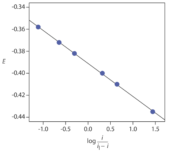
If a reaction is electrochemically reversible, a plot of E versus \(\log \frac{i}{i_l - i}\) is a straight line with a slope of –0.05916/n. In addition, the slope should yield an integer value for n.
The following data were obtained from a linear scan hydrodynamic voltammogram of a reversible reduction reaction.
| E (V vs. SCE) | current (μA) |
|---|---|
| –0.358 | 0.37 |
| –0.372 | 0.95 |
| –0.382 | 1.71 |
| –0.400 | 3.48 |
| –0.410 | 4.20 |
| –0.435 | 4.97 |
The limiting current is 5.15 μA. Show that the reduction reaction is reversible, and determine values for n and for E1/2.
Solution
Figure \(\PageIndex{3}\) shows a plot of E versus \(\log \frac{i}{i_l - i}\). Because the result is a straight-line, we know the reaction is electrochemically reversible under the conditions of the experiment. A linear regression analysis gives the equation for the straight line as
\[E=-0.391 \mathrm{V}-0.0300 \log \frac{i}{i_{l}-i} \nonumber \]
From Equation \ref{app3}, the slope is equivalent to –0.05916/n; solving for n gives a value of 1.97, or 2 electrons. From Equation \ref{app3} we also know that E1/2 is the y-intercept for a plot of E versus \(\log \frac{i}{i_l - i}\); thus, E1/2 for the data in this example is –0.391 V versus the SCE.
We also can use cyclic voltammetry to evaluate electrochemical reversibility by looking at the difference between the peak potentials for the anodic and the cathodic scans. For an electrochemically reversible reaction, the following equation holds true.
\[\Delta E_{p}=E_{p, a}-E_{p, c}=\frac{0.05916 \ \mathrm{V}}{n} \label{app4} \]
As an example, for a two-electron reduction we expect a \(\Delta E_p\) of approximately 29.6 mV. For an electrochemically irreversible reaction the value of \(\Delta E_p\) is larger than expected.
Determining Equilibrium Constants for Coupled Chemical Reactions
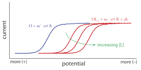
Another important application of voltammetry is determining the equilibrium constant for a solution reaction that is coupled to a redox reaction. The presence of the solution reaction affects the ease of electron transfer in the redox reaction, shifting E1/2 to a more negative or to a more positive potential. Consider, for example, the reduction of O to R
\[O+n e^{-} \rightleftharpoons R \label{app5} \]
the voltammogram for which is shown in Figure \(\PageIndex{4}\). If we introduce a ligand, L, that forms a strong complex with O, then we also must consider the reaction
\[O+p L\rightleftharpoons O L_{p} \label{app6} \]
In the presence of the ligand, the overall redox reaction is
\[O L_{p}+n e^{-} \rightleftharpoons R+p L \label{app7} \]
Because of its stability, the reduction of the OLp complex is less favorable than the reduction of O. As shown in Figure \(\PageIndex{4}\), the resulting voltammogram shifts to a potential that is more negative than that for O. Furthermore, the shift in the voltammogram increases as we increase the ligand’s concentration.
We can use this shift in the value of E1/2 to determine both the stoichiometry and the formation constant for a metal-ligand complex. To derive a relationship between the relevant variables we begin with two equations: the Nernst equation for the reduction of O
\[E=E_{O / R}^{\circ}-\frac{0.05916}{n} \log \frac{[R]_{x=0}}{[O]_{x=0}} \label{app8} \]
and the stability constant, \(\beta_p\) for the metal-ligand complex at the electrode surface.
\[\beta_{p} = \frac{\left[O L_p\right]_{x = 0}}{[O]_{x = 0}[L]_{x = 0}^p} \label{app9} \]
In the absence of ligand the half-wave potential occurs when [R]x = 0 and [O]x = 0 are equal; thus, from the Nernst equation we have
\[\left(E_{1 / 2}\right)_{n c}=E_{O / R}^{\circ} \label{app10} \]
where the subscript “nc” signifies that the complex is not present. When ligand is present we must account for its effect on the concentration of O. Solving Equation \ref{app9} for [O]x = 0 and substituting into the Equation \ref{app8} gives
\[E=E_{O/R}^{\circ}-\frac{0.05916}{n} \log \frac{[R]_{x=0}[L]_{x=0}^{p} \beta_{p}}{\left[O L_{p}\right]_{x=0}} \label{app11} \]
If the formation constant is sufficiently large, such that essentially all O is present as the complex OLp, then \([R]_{x = 0}\) and \([OL_p]_{x = 0}\) are equal at the half-wave potential, and Equation \ref{app11} simplifies to
\[\left(E_{1 / 2}\right)_{c} = E_{O/R}^{\circ} - \frac{0.05916}{n} \log{} [L]_{x=0}^{p} \beta_{p} \label{app12} \]
where the subscript “c” indicates that the complex is present. Defining \(\Delta E_{1/2}\) as
\[\triangle E_{1 / 2}=\left(E_{1 / 2}\right)_{c}-\left(E_{1 / 2}\right)_{n c} \label{app13} \]
and substituting Equation \ref{app10} and Equation \ref{app12} and expanding the log term leaves us with the following equation.
\[\Delta E_{1 / 2}=-\frac{0.05916}{n} \log \beta_{p}-\frac{0.05916 p}{n} \log {[L]} \label{app14} \]
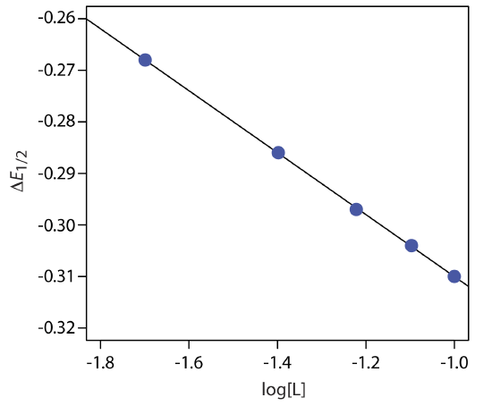
A plot of \(\Delta E_{1/2}\) versus log[L] is a straight-line, with a slope that is a function of the metal-ligand complex’s stoichiometric coefficient, p, and a y-intercept that is a function of its formation constant \(\beta_p\).
A voltammogram for the two-electron reduction (n = 2) of a metal, M, has a half-wave potential of –0.226 V versus the SCE. In the presence of an excess of ligand, L, the following half-wave potentials are recorded.
| [L] (M) | (E1/2)c (V vs. SCE) |
|---|---|
| 0.020 | –0.494 |
| 0.040 | –0.512 |
| 0.060 | –0.523 |
| 0.080 | –0.530 |
| 0.100 | –0.536 |
Determine the stoichiometry of the metal-ligand complex and its formation constant.
Solution
We begin by calculating values of \(\Delta E_{1/2}\) using Equation \ref{app13}, obtaining the values in the following table.
| [L] (M) | \(\Delta E_{1/2}\) (V vs. SCE) |
|---|---|
| 0.020 | –0.268 |
| 0.040 | –0.286 |
| 0.060 | –0.297 |
| 0.080 | –0.304 |
| 0.100 | –0.310 |
Figure \(\PageIndex{5}\) shows the resulting plot of \(\Delta E_{1/2}\) as a function of log[L]. A linear regression analysis gives the equation for the straight line as
\[\triangle E_{1 / 2}=-0.370 \mathrm{V}-0.0601 \log {[L]} \nonumber \]
From Equation \ref{app14} we know that the slope is equal to –0.05916p/n. Using the slope and n = 2, we solve for p obtaining a value of 2.03 ≈ 2. The complex’s stoichiometry, therefore, is ML2. We also know, from Equation \ref{app14}, that the y-intercept is equivalent to –(0.05916/n)log\(\beta_p\). Solving for \(\beta_2\) gives a formation constant of \(3.2 \times 10^{12}\).
Cyclic voltammetry is one of the most powerful electrochemical techniques for exploring the mechanism of coupled electrochemical and chemical reactions. The treatment of this aspect of cyclic voltammetry is beyond the level of this text, although you can consult this chapter’s additional resources for additional information.