23.5: Instruments for Measuring Cell Potentials

To measure the potential of an electrochemical cell in a way that draws essentially no current we use a potentiometer. To help us understand how a potentiometer accomplishes this, we will describe the instrument as if the analyst is operating it manually. To do so the analyst observes a change in the current or the potential and manually adjusts the instrument’s settings to maintain the desired experimental conditions. It is important to understand that modern electrochemical instruments provide an automated, electronic means for controlling and measuring current and potential, and that they do so by using very different electronic circuitry than that described here.

Figure \(\PageIndex{1}\). Schematic diagram of a manual potentiometer: C is the reference electrode; W is the working electrode; SW is a slide-wire resistor; T is a tap key and i is an ammeter for measuring current.

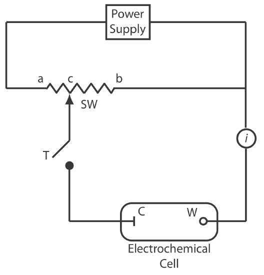
Figure \(\PageIndex{1}\) shows a schematic diagram for a manual potentiometer that consists of a power supply, an electrochemical cell with a working electrode and a counter electrode, an ammeter to measure the current that passes through the electrochemical cell, an adjustable, slide-wire resistor, and a tap key for closing the circuit through the electrochemical cell. Using Ohm’s law, the current in the upper half of the circuit is

\[i_{\text {upper}}=\frac{E_{\mathrm{PS}}}{R_{a b}} \label{pot1} \]

where E_PS is the power supply’s potential, and R_ab is the resistance between points a and b of the slide-wire resistor. In a similar manner, the current in the lower half of the circuit is

\[i_{\text {lower}}=\frac{E_{\text {cell}}}{R_{c b}} \label{pot2} \]

where E_cell is the potential difference between the working electrode and the counter electrode, and R_cb is the resistance between the points c and b of the slide-wire resistor. When i_upper = i_lower = 0, no current flows through the ammeter and the potential of the electrochemical cell is

\[E_{\mathrm{coll}}=\frac{R_{c b}}{R_{a b}} \times E_{\mathrm{PS}} \label{pot3} \]

To determine E_cell we briefly press the tap key and observe the current at the ammeter. If the current is not zero, then we adjust the slide wire resistor and remeasure the current, continuing this process until the current is zero. When the current is zero, we use Equation \ref{pot3} to calculate E_cell.

Using the tap key to briefly close the circuit through the electrochemical cell minimizes the current that passes through the cell and limits the change in the electrochemical cell’s composition. For example, passing a current of 10^–9 A through the electrochemical cell for 1 s changes the concentrations of species in the cell by approximately 10^–14 moles.

\[10^{-9} \text{ A} = 10^{-9} \text{ C/s} \label{pot4} \]

\[10^{-9} \text{ C/s} \times 1 \text{ s} \times \frac {1 \text{ mol}} {96485 \text{C}} = 1.0 \times 10^{-14} \text{ mol} \label{pot5} \]

Of course, trying to measure a potential in this way is tedious. Modern potentiometers use operational amplifiers to create a high-impedance voltmeter that measures the potential while drawing a current of less than \(10^{–9}\) A. The relative error, \(E_r\), in the measured potential

\[E_r = \frac {R_\text{cell}} {R_\text{meter} + R_\text{cell}} \label{pot6} \]

where \(R_\text{cell}\) is the resistance of the solution in the electrochemical cell and \(R_\text{meter}\) is the resistance of the meter. For a solution with a resistance of \(10 \text{M}\Omega\) to achieve a relative error of \(-0.1\%)\) or \(-0.001\) requires an \(R_\text{meter}\) of

\[-0.001 = \frac {-10 \text{ M}\Omega} {R_\text{meter} + 10 \text{ M}\Omega} \nonumber \]

\[-0.001 \times R_\text{meter} - 0.01 = -10 \text{ M}\Omega \nonumber \]

\[-0.001 \times R_\text{meter} = -9.990 \text{ M}\Omega \nonumber \]

\[R_\text{meter} = 9990 \text{ M}\Omega \nonumber \]