23.6: Quantitative Potentiometry

The most important application of potentiometry is determining the concentration of an analyte in solution. Most potentiometric electrodes are selective toward the free, uncomplexed form of the analyte, and do not respond to any of the analyte’s complexed forms. This selectivity provides potentiometric electrodes with a significant advantage over other quantitative methods of analysis if we need to determine the concentration of free ions. For example, calcium is present in urine both as free Ca²⁺ ions and as protein-bound Ca²⁺ ions. If we analyze a urine sample using atomic absorption spectroscopy, the signal is propor- tional to the total concentration of Ca²⁺ because both free and bound calcium are atomized. Analyzing urine with a Ca²⁺ ISE, however, gives a signal that is a function of only free Ca²⁺ ions because the protein-bound Ca²⁺ can not interact with the electrode’s membrane. In this section, we consider several important aspects of quantiative potentiometry.

The Relationship Between Concentration and Potential

In Chapter 23.3, we showed that the potential of an ion-selective electrode for an ion with a charge of z is

\[E_{\mathrm{cell}}=K+\frac{0.05916}{z} \log \left(a_{A}\right)_{\mathrm{samp}} \label{quant1} \]

where K is a constant that includes the potentials of the ion-selective electrode's internal and external reference electrodes, any asymmetry potential associated with the ion-selective electrode's membrane, and the analyte's activity in the ion-selective electrode's internal solution. Equation \ref{quant1} is a general equation and applies to all types of ion-selective electrodes. Note that when the analyte is a cation, an increase in the analyte's activity results in results in an increase in the potential; when the analyte is an anion, which makes z a negative number, an increase in the analyte's activity results in a decrease in the potential.

As the concentrations of ions in solution often are reported as pX values, where

\[\text{pX} = - \log a_\text{X} \label{quant2} \]

it is convenient to substitute Equation \ref{quant2} into Equation \ref{quant1}

\[E_{\mathrm{cell}}=K - \frac{0.05916}{z} \text{ pA} \label{quant3} \]

Note that for a cation, an increase in pA results in a decrease in the potential; when the analyte is an anion, an increase in pA results in an increase in the potential.

Calibrating Potentiometric Electrodes

To use Equation \ref{quant3} we need to determine the value of K, which we can do using one or more external standards or by the method of standard addition, both of which were covered in Chapter 1.5. One complication, of course, is that potential is a function of the analyte's activity instead of its concentration.

Activity and Concentration

Equation \ref{quant1} is written in terms of the analyte's activity. When we use a potentiometric electrode, however, our goal is to determine the analyte’s concentration. As we learned in Chapter 22, an ion’s activity is the product of its concentration, [Mⁿ⁺], and a matrix-dependent activity coefficient, \(\gamma_{Mn^{n+}}\).

\[a_{M^{n+}}=\left[M^{n+}\right] \gamma_{M^{n+}} \label{quant4} \]

Substituting Equation \ref{quant4} into Equation \ref{quant1} and rearranging, gives

\[E_{\mathrm{cell}}=K+\frac{0.05916}{n} \log \gamma_{M^{n+}}+\frac{0.05916}{n} \log \left[M^{n+}\right] \label{quant5} \]

We can solve Equation \ref{quant5} for the metal ion’s concentration if we know the value for its activity coefficient. Unfortunately, if we do not know the exact ionic composition of the sample’s matrix—which is the usual situation—then we cannot calculate the value of \(\gamma_{Mn^{n+}}\). There is a solution to this dilemma. If we design our system so that the standards and the samples have an identical matrix, then the value of \(\gamma_{Mn^{n+}}\) remains constant and Equation \ref{quant5} simplifies to

\[E_{\mathrm{cell}}=K^{\prime}+\frac{0.05916}{n} \log \left[M^{n+}\right] \label{quanat6} \]

where \(K^{\prime}\) includes the activity coefficient.

Calibration Using External Standards

In the absence of interferents, a calibration curve of E_cell versus loga_A, where A is the analyte, is a straight-line. A plot of E_cell versus log[A], however, may show curvature at higher concentrations of analyte as a result of a matrix-dependent change in the analyte’s activity coefficient. To maintain a consistent matrix we add a high concentration of an inert electrolyte to all samples and standards. If the concentration of added electrolyte is sufficient, then the difference between the sample’s matrix and the matrix of the standards will not affect the ionic strength and the activity coefficient essentially remains constant. The inert electrolyte added to the sample and the standards is called a total ionic strength adjustment buffer (TISAB).

Example \(\PageIndex{1}\)

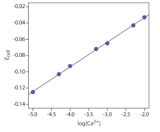
The concentration of Ca²⁺ in a water sample is determined using the method of external standards. The ionic strength of the samples and the standards is maintained at a nearly constant level by making each solution 0.5 M in KNO₃. The measured cell potentials for the external standards are shown in the following table.

[Ca^2^+] (M)	Ecell (V)
\(1.00 \times 10^{-5}\)	–0.125
\(5.00 \times 10^{-5}\)	–0.103
\(1.00 \times 10^{-4}\)	–0.093
\(5.00 \times 10^{-4}\)	–0.072
\(1.00 \times 10^{-3}\)	–0.063
\(5.00 \times 10^{-3}\)	–0.043
\(1.00 \times 10^{-2}\)	–0.033

What is the concentration of Ca²⁺ in a water sample if its cell potential is found to be –0.084 V?

Solution

Linear regression gives the calibration curve in Figure \(\PageIndex{1}\), with an equation of

\[E_{\mathrm{cell}}=0.027+0.0303 \log \left[\mathrm{Ca}^{2+}\right] \nonumber \]

Substituting the sample’s cell potential gives the concentration of Ca²⁺ as \(2.17 \times 10^{-4}\) M. Note that the slope of the calibration curve, which is 0.0303, is slightly larger than its ideal value of 0.05916/2 = 0.02958; this is not unusual and is one reason for using multiple standards. One reason that it is not unusual to find that the experimental slope deviates from its ideal value of 0.05916/n is that this ideal value assumes that the temperature is 25°C.

Figure \(\PageIndex{1}\). Calibration curve for the data in Example \(\PageIndex{1}\).

Calibration Using Standard Additions

Another approach to calibrating a potentiometric electrode is the method of standard additions, which was introduced in Chapter 1.5. First, we transfer a sample with a volume of V_samp and an analyte concentration of C_samp into a beaker and measure the potential, (E_cell)_samp. Next, we make a standard addition by adding to the sample a small volume, V_std, of a standard that contains a known concentration of analyte, C_std, and measure the potential, (E_cell)_std. If V_std is significantly smaller than V_samp, then we can safely ignore the change in the sample’s matrix and assume that the analyte’s activity coefficient is constant. Example \(\PageIndex{9}\) demonstrates how we can use a one-point standard addition to determine the concentration of analyte in a sample.

Example \(\PageIndex{2}\)

The concentration of Ca²⁺ in a sample of sea water is determined using a Ca ion-selective electrode and a one-point standard addition. A 10.00-mL sample is transferred to a 100-mL volumetric flask and diluted to volume. A 50.00-mL aliquot of the sample is placed in a beaker with the Ca ISE and a reference electrode, and the potential is measured as –0.05290 V. After adding a 1.00-mL aliquot of a \(5.00 \times 10^{-2}\) M standard solution of Ca²⁺ the potential is –0.04417 V. What is the concentration of Ca²⁺ in the sample of sea water?

Solution

To begin, we write the Nernst equation before and after adding the standard addition. The cell potential for the sample is

\[\left(E_{\mathrm{cell}}\right)_{\mathrm{samp}}=K+\frac{0.05916}{2} \log C_{\mathrm{samp}} \nonumber \]

and that following the standard addition is

\[\left(E_{\mathrm{cell}}\right)_{\mathrm{std}}=K+\frac{0.05916}{2} \log \left\{ \frac {V_\text{samp}} {V_\text{tot}}C_\text{samp} + \frac {V_\text{std}} {V_\text{tot}}C_\text{std} \right\} \nonumber \]

where V_tot is the total volume (V_samp + V_std) after the standard addition. Subtracting the first equation from the second equation gives

\[\Delta E = \left(E_{\mathrm{cell}}\right)_{\mathrm{std}} - \left(E_{\mathrm{cell}}\right)_{\mathrm{samp}} = \frac{0.05916}{2} \log \left\{ \frac {V_\text{samp}} {V_\text{tot}}C_\text{samp} + \frac {V_\text{std}} {V_\text{tot}}C_\text{std} \right\} - \frac{0.05916}{2}\log C_\text{samp} \nonumber \]

Rearranging this equation leaves us with

\[\frac{2 \Delta E_{cell}}{0.05916} = \log \left\{ \frac {V_\text{samp}} {V_\text{tot}} + \frac {V_\text{std}C_\text{std}} {V_\text{tot}C_\text{samp}} \right\} \nonumber \]

Substituting known values for \(\Delta E\), V_samp, V_std, V_tot and C_std,

\[\begin{array}{l}{\frac{2 \times\{-0.04417-(-0.05290)\}}{0.05916}=} \\ {\log \left\{\frac{50.00 \text{ mL}}{51.00 \text{ mL}}+\frac{(1.00 \text{ mL})\left(5.00 \times 10^{-2} \mathrm{M}\right)}{(51.00 \text{ mL}) C_{\mathrm{samp}}}\right\}} \\ {0.2951=\log \left\{0.9804+\frac{9.804 \times 10^{-4}}{C_{\mathrm{samp}}}\right\}}\end{array} \nonumber \]

and taking the inverse log of both sides gives

\[1.973=0.9804+\frac{9.804 \times 10^{-4}}{C_{\text {samp }}} \nonumber \]

Finally, solving for C_samp gives the concentration of Ca²⁺ as \(9.88 \times 10^{-4}\) M. Because we diluted the original sample of seawater by a factor of 10, the concentration of Ca²⁺ in the seawater sample is \(9.88 \times 10^{-3}\) M.

The Operational Definition of pH

With the availability of inexpensive glass pH electrodes and pH meters, the determination of pH is one of the most common quantitative analytical measurements. The potentiometric determination of pH, however, is not without complications, several of which we discuss in this section.

One complication is confusion over the meaning of pH [Kristensen, H. B.; Saloman, A.; Kokholm, G. Anal. Chem. 1991, 63, 885A–891A]. The conventional definition of pH in most general chemistry textbooks is given in terms of the concentration of H⁺

\[\mathrm{pH}=-\log \left[\mathrm{H}^{+}\right] \label{quant7} \]

As we now know, when we measure pH it actually is a measure of the activity of H⁺.

\[\mathrm{pH}=-\log a_{\mathrm{H}^{+}} \label{quant8} \]

Try this experiment—find several general chemistry textbooks and look up pH in each textbook’s index. Turn to the appropriate pages and see how it is defined. Next, look up activity or activity coefficient in each textbook’s index and see if these terms are indexed.

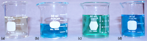
Equation \ref{quant7} only approximates the true pH. If we calculate the pH of 0.1 M HCl using Equation \ref{quant7}, we obtain a value of 1.00; the solution’s actual pH, as defined by Equation \ref{quant8}, is 1.1 [Hawkes, S. J. J. Chem. Educ. 1994, 71, 747–749]. The activity and the concentration of H⁺ are not the same in 0.1 M HCl because the activity coefficient for H⁺ is not 1.00 in this matrix. Figure \(\PageIndex{2}\) shows a more colorful demonstration of the difference between activity and concentration.

Figure \(\PageIndex{2}\). A demonstration of the difference between activity and concentration using the indicator methyl green. The indicator is pale yellow in its acid form (beaker a: 1.0 M HCl) and is blue in its base form (beaker d: H₂O). In 10 mM HCl the indicator is in its base form (beaker b: 20 mL of 10 mM HCl with 3 drops of methyl green). Adding 20 mL of 5 M LiCl to this solution shifts the indicator's color to green (beaker c); although the concentration of HCl is cut in half to 5 mM, the activity of H⁺ has increased as evidenced by the green color that is intermediate between the indicator’s pale yellow, acid form and its blue, base form. The demonstration shown here is adapted from McCarty, C. G.; Vitz, E. “pH Paradoxes: Demonstrating That It Is Not True That pH ≡ –log[H⁺],” J. Chem. Educ. 2006, 83, 752–757. This paper provides several additional demonstrations that illustrate the difference between concentration and activity.

A second complication in measuring pH is the uncertainty in the relationship between potential and activity. For a glass membrane electrode, the cell potential, (E_cell)_samp, for a sample of unknown pH is

\[(E_{\text{cell}})_\text {samp} = K-\frac{R T}{F} \ln \frac{1}{a_{\mathrm{H}^{+}}}=K-\frac{2.303 R T}{F} \mathrm{pH}_{\mathrm{samp}} \label{quant9} \]

where K includes the potential of the reference electrode, the asymmetry potential of the glass membrane, and any junction potentials in the electrochemical cell. All the contributions to K are subject to uncertainty, and may change from day-to-day, as well as from electrode-to-electrode. For this reason, before using a pH electrode we calibrate it using a standard buffer of known pH. The cell potential for the standard, (E_cell)_std, is

\[\left(E_{\text {ccll}}\right)_{\text {std}}=K-\frac{2.303 R T}{F} \mathrm{p} \mathrm{H}_{\mathrm{std}} \label{quant10} \]

where pH_std is the standard’s pH. Subtracting Equation \ref{quan10} from Equation \ref{quant9} and solving for pH_samp gives

\[\text{pH}_\text{samp} = \text{pH}_\text{std} - \frac{\left\{\left(E_{\text {cell}}\right)_{\text {samp}}-\left(E_{\text {cell}}\right)_{\text {std}}\right\} F}{2.303 R T} \label{quant11} \]

which is the operational definition of pH adopted by the International Union of Pure and Applied Chemistry [Covington, A. K.; Bates, R. B.; Durst, R. A. Pure & Appl. Chem. 1985, 57, 531–542].

Calibrating a pH electrode presents a third complication because we need a standard with an accurately known activity for H⁺. Table \(\PageIndex{1}\) provides pH values for several primary standard buffer solutions accepted by the National Institute of Standards and Technology.

Table \(\PageIndex{1}\). pH Values for Selected NIST Primary Standard Buffers

temp (^oC)	saturated (at 25^oC) KHC4H4O7 (tartrate)	0.05 m KH2C6H5O7 (citrate)	0.05 m KHC8H4O4 (phthlate)	0.025 m KH2PO4, 0.025 m NaHPO4	0.008695 m KH2PO4, 0.03043 m Na2HPO4	0.01 m Na4B4O7	0.025 m NaHCO3, 0.025 m Na2CO3
0	—	3.863	4.003	6.984	7.534	9.464	10.317
5	—	3.840	3.999	6.951	7.500	9.395	10.245
10	—	3.820	3.998	6.923	7.472	9.332	10.179
15	—	3.802	3.999	6.900	7.448	9.276	10.118
20	—	3.788	4.002	6.881	7.429	9.225	10.062
25	3.557	3.776	4.008	6.865	7.413	9.180	10.012
30	3.552	3.766	4.015	6.854	7.400	9.139	9.966
35	3.549	3.759	4.024	6.844	7.389	9.012	9.925
40	3.547	3.753	4.035	6.838	7.380	9.068	9.889
45	3.547	3.750	4.047	6.834	7.373	9.038	9.856
50	3.549	3.749	4.060	6.833	7.367	9.011	9.828
Source: Values taken from Bates, R. G. Determination of pH: Theory and Practice, 2nd ed. Wiley: New York, 1973. See also Buck, R. P., et. al.“Measurement of pH. Definition, Standards, and Procedures,” Pure. Appl. Chem. 2002, 74, 2169–2200. All concentrations are molal (m).

To standardize a pH electrode using two buffers, choose one near a pH of 7 and one that is more acidic or basic depending on your sample’s expected pH. Rinse your pH electrode in deionized water, blot it dry with a laboratory wipe, and place it in the buffer with the pH closest to 7. Swirl the pH electrode and allow it to equilibrate until you obtain a stable reading. Adjust the “Standardize” or “Calibrate” knob until the meter displays the correct pH. Rinse and dry the electrode, and place it in the second buffer. After the electrode equilibrates, adjust the “Slope” or “Temperature” knob until the meter displays the correct pH.

Some pH meters can compensate for a change in temperature. To use this feature, place a temperature probe in the sample and connect it to the pH meter. Adjust the “Temperature” knob to the solution’s temperature and calibrate the pH meter using the “Calibrate” and “Slope” controls. As you are using the pH electrode, the pH meter compensates for any change in the sample’s temperature by adjusting the slope of the calibration curve using a Nernstian response of 2.303RT/F.