21.2: Spectroscopic Surface Methods

In this section we consider three representative surface analytical methods: X-ray photoelectron spectroscopy, in which the input is a beam of X-ray photons and the output is electrons; Auger electron spectroscopy, in which the input is either a beam of electrons or of X-ray photons and the output is electrons; and secondary-ion mass spectrometry, in which the input is a beam of ions and the output is ions.

X-Ray Photoelectron Spectroscopy (XPS)

In X-ray photoelectron spectroscopy, which is also known as electron spectroscopy for chemical analysis (ESCA), we measure the kinetic energy of electrons ejected from a sample following the absorption of X-ray photons. The resulting spectrum is a count of these emitted electrons as a function of their energy.

Principles of XPS

We can explain the origin of X-ray photoelectron spectroscopy using the photoelectric effect. Figure \(\PageIndex{1}a\) shows the energy level diagram for an element's 1s, 2s, and 2p core-level electrons along with their KLM designations (see Chapter 12.1 for a previous discussion of this way of designating electrons). A nearly monoenergetic X-ray beam of known energy is focused on the sample, which results in the ejection of a core-level photoelectron, as shown in Figure \(\PageIndex{1}b\). The kinetic energy of this emitted electron, \(E_{KE}\), is related to its binding energy to the nucleus, \(E_{BE}\), by the equation

\[E_{KE} = h \nu - E_{EB} - \Phi_w \label{xps1} \]

where \(h \nu\) is the energy of the X-ray photon and \(\Phi_w\) is the spectrometer's work function (the energy needed to remove the electron from the surface and into the vacuum). The most common sources of X-rays are the Mg \(K_{\alpha}\) line with an energy of 1253.6 eV or the Al \(K{\alpha}\) line with an energy of 1486.6 eV.

The core-level vacancy created by the photoelectron leaves the atom with an unstable electron configuration. Relaxation to the ground state occurs when this vacancy is filled by an electron from a higher energy shell, with the excess energy released as either the emission of a second electron or the fluorescent emission of a characteristic X-ray, as seen in Figure \(\PageIndex{1}c\). The secondary electron in Figure \(\PageIndex{1}c\) is called an Auger electron.

Figure \(\PageIndex{1}\): Energy level diagrams for X-ray photoelectron spectroscopy. In (a) we see the 1s, 2s, and 2p electrons along with their KLM designations. When a photon of sufficient energy is absorbed by the sample (b), a core-level electron is ejected as a photoelectron leaving an unstable electron configuration in which there is a vacancy in the 1s orbital. In (c) an electron from a higher energy orbital moves into the vacancy created by the initial photon with the remaining energy released as a secondary electron or as an X-ray photon.

Figure \(\PageIndex{2}\) provides an example of an XPS survey spectrum for aluminum oxide, \(\ce{Al2O3}\), using the \(K_{\alpha}\) line for aluminum as the source of X-rays. The peak table gives the binding energies of the peaks for aluminum and for oxygen using the \(K_{\alpha}\) for Al and, for comparison, the \(K_{\alpha}\) line for Mg. Note the difference in how the major peaks are labeled. The photoelectrons ejected in the process shown in Figure \(\PageIndex{1}b\) are designated by the element and the ns notation that specifies the orbital from which the electron was ejected. Auger electrons are designated using the KLM notation, specifying the initial vacancy created by the absorbed photon, the source of the electron that fills that vacancy, and the source of the ejected Auger electron. The O_KLL peak in this spectrum is consistent with the scheme shown in Figure \(\PageIndex{1}c\). When the source of the second and third electrons is from the valance shell, then notation is sometimes written as KVV; the O_KLL peak here could be designated as O_KVV.

Figure \(\PageIndex{2}\): The XPS spectrum for \(\ce{Al2O3}\) using the Al \(K_{\alpha}\) line, with the major peaks labeled. A spectrum such as this, which spans a wide range of energies, is called a survey spectrum. The source of each peak is shown above or next to the spectrum's peaks. The peak table provides the binding energies for aluminum and for oxygen using both the \(K_{\alpha}\) for Al and the \(K_{\alpha}\) for Mg. The original data used to create this figure is from the xpslibrary.

There are a few additional interesting features to note in the survey spectrum for Al₂O₃. One is the presence of a peak for carbon even though the sample, Al₂O₃, does not contain carbon. The prevalence of carbon in the atmosphere means that trace levels of carbon appear in almost all XPS spectra.

A second feature is the increase in the signal on the high binding energy (low kinetic energy) side of peaks, which is particularly visible here for the O_1s peak the C_1s peak, and the Al_2s peak. The source of this background is electrons that fail to escape the sample without undergoing inelastic collisions that result in a loss of kinetic energy and, given Equation \ref{xps1}, are recorded as if they have a larger than expected binding energy. Because X-rays penetrate more deeply into the sample than the depth from which electrons can travel without undergoing an inelastic collision, this background is unavoidable. Note that the background is more significant at higher binding energies (smaller kinetic energies).

A third feature is that the binding energy of an XPS peak is independent of the X-ray source, but the binding energy for an Auger peak varies with the X-ray source's energy (see table in Figure \(\PageIndex{2}\)). The kinetic energy of the O_1s, Al_2s, and Al_2p photoelectrons is the difference between the energy of the X-ray photon, \(h \nu\), and each electron's binding energy, BE; if we change the X-ray source, then \(h \nu\) and KE increase in value, but the BE remains fixed. For the O_KLL Auger electron, the kinetic energy depends on the difference in the binding energies of the three electrons involved

\[\text{KE} \approx \text{BE}_K - \text{BE}_L - \text{BE}_L \label{xps2} \]

and is, therefore, independent of the energy of the X-ray source. Given Equation \ref{xps1}, if the KE remains constant, then an increase in the energy of the X-ray photon, \(h \nu\), means that the apparent BE must increase. This shift in binding energy when using a different source is one way to identify a peak as resulting from Auger electrons.

Instrumentation

The basic instrumentation for XPS is shown in Figure \(\PageIndex{3}\). The most common X-ray sources, as noted above, are Mg (1253.6 eV) and Al (1486.6 ev), which have the advantage of relatively narrow line-widths (0.7 and 0.9 eV, respectively) and, therefore, a relatively narrow range of energies. Higher energy sources are available, such as Ag (2984.4 ev), but at the cost of a wider line-width (2.6 eV). A system of electron lenses collects and focuses the ejected electrons onto the entrance slit of a hemispherical analyzer. The path of an electron through the analyzer depends upon its kinetic energy. By varying the potentials applied to the hemispherical analyzer's inner and outer plates, electrons of different kinetic energies reach the detector. A sputtering gun is an optional feature that can be used to clean the surface of the sample or to remove successive layers of the sample, allowing for the gathering of spectra at various depths within the sample. Calibration of the spectrometer's binding energy scale, which accounts for the spectrometer's work function, is made using specific lines for one or more conductive metals; examples include Au 4f_7/2 at 83.95 eV and Cu 2p_3/2 at 932.63 ev. The peak for carbon that appears in almost all XPS spectra provides an additional way to check the calibration of the binding energy scale.

Figure \(\PageIndex{3}\): Schematic diagram of the basic instrumentation for X-ray photoelectron spectroscopy: an X-ray source for generating photoelectrons; a sputtering gun for cleaning the sample's surface or for removing layers of the sample; a set of electron lenses for collecting and focusing the photoelectrons; a hemispherical analyzer for isolating electrons by their kinetic energies; and a transducer to count electrons. The entire instrument is held under a vacuum.

Applications

X-ray photoelectron spectroscopy is a particularly useful tool for determining the composition and structure of a sample. XPS also can provide information about how the composition of a sample varies with depth and quantitative information about a sample's components.

Qualitative Analysis. One of the strengths of X-ray photoelectron spectroscopy is the ability to determine the elements that make up a sample's surface. Figure \(\PageIndex{4}\) shows a survey scan from 0 eV to 1100 eV of a ceramic material. In addition to the O1s peak, we see strong peaks for Si and Al—probably an aluminosilicate ceramic—and small peaks for a variety of elements: La, Ba, Mn, Sn, Ca, Cl, P, and Mg. NIST maintains an extensive, and searchable, database of XPS peaks that help in identifying the elements in a sample.

Figure \(\PageIndex{4}\): X-ray photoelectron survey spectrum for an unidentified ceramic material showing the peak assignments, which include major elements that we might reasonably expect from a ceramic (oxygen, magnesium, aluminum, calcium, and silicon) and a variety of trace elements (lanthinum, barium, manganese, tin, chlorine, and phosphorous). The original data used to create this figure is from the xpslibrary.

Chemical Shifts. An element's binding energy is sensitive to its chemical environment, particularly with respect to oxidation states and structure. For example, Table \(\PageIndex{1}\) provides the binding energy for chlorine's 2p line in three potassium salts drawn from the NIST database with all values from the same literature source. Using KCl, in which chlorine has an oxidation state of –1, as a baseline, the Cl 2p peak for KClO₃ is shifted by +8.4 eV and the Cl 2p peak for KClO₄ is shifted by +10.3 eV. The direction of the shift makes sense, as we expect that it will require more energy to remove an electron from an element that has a more positive oxidation state.

Table \(\PageIndex{1}\). Binding energies for the Cl 2p XPS peak as a function of chlorine's oxidation state.

compound	oxidation state for chlorine	binding energy (eV) for Cl 2p line	\(\Delta \text{BE}\) relative to KCl
KCl	–1	198.1	—
KClO3	+5	206.5	+8.4
KClO4	+7	208.4	+10.3

Chemical shifts also reflect changes in chemical structure. Figure \(\PageIndex{5}\), for example, shows a high resolution scan for the oxygen 2p peak for same sample of aluminum oxide, Al₂O₃, in Figure \(\PageIndex{1}\). The surface of a metal oxide often has three distinct sources of oxygen: oxides, which make up the bulk of the sample, hydroxides that form at the surface following the chemisorption of water, and water that is physically absorbed to the surface. Curve-fitting of the raw data shows the contribution of each type of oxygen to the raw data and, through the peak areas, their relative abundance.

Figure \(\PageIndex{5}\): The results of curve-fitting to determine the relative contribution of different sources of oxygen—oxides, hydroxides, and water—to the O_2p peak for aluminum oxide. The original data used to create this figure is from the xpslibrary.

Wagner Plots. Both the binding energy of an X-ray photoelectron and the kinetic energy of an Auger electron convey information about the element from which the electrons were emitted. A Wagner plot shows both the binding energy for a photoelectron that leaves a particular core-level vacancy and the kinetic energy of the Auger electron whose origin arises from the filling of this core-level vacancy. Figure \(\PageIndex{6}\) shows an example of a Wagner plot for copper based on its 2p_3/2 X-ray photoelectron and its LMM Auger electron. The diagonal lines are called the modified Auger parameter, which is defined as the sum of the XPS binding energy and the AES kinetic energy. Values for 20 compounds are included in this plot. Of interest here is the clustering of the individual compounds. For example, all of the samples for which copper has an oxidation state of +1 (shown as magenta squares) have similar binding energies between 932 eV and 933 eV, but with more variable kinetic energies, which range from 914 eV to 917 eV. Most of the compounds in which copper has an oxidation state of +2 (shown as blue diamonds) have modified Auger parameters between approximately 1850 eV and 1851 eV, although there is signifiant variation in their individual binding energies and kinetic energies. The two metals (shown as green circles) and the commpounds CuS and CuSe occupy a similar space within the Wagner plot. Interestingly, both CuS and CuSe are transition metal chalcogenides and have semiconducting properties.

Figure \(\PageIndex{6}\): Wagner plot for 20 copper compounds. The raw data is from https://srdata.nist.gov/xps/Default.aspx and includes 140 measurements of binding energies and 99 measurements of kinetic energies. Compounds are identified by the oxidation state of copper.

Information at Depth. X-rays penetrate into a sample to a depth that is greater than the distance the photoelectron can travel without losing energy to inelastic collisions. We can take advantage of this to vary the depth from which we gather information. Figure \(\PageIndex{7}\) shows how this is accomplished by changing the angle from which we collect and analyze photoelectrons. The length of the solid black line is the distance an electron can travel without losing energy in an inelastic collision. When the detector is placed at 90° to the sample's surface, the sampling depth is at its greatest. Adjusting the detector so that it is at 30° to the surface, results in its detecting electrons from a depth that is just half of that when the detector is at 90°.

Figure \(\PageIndex{7}\): Illustration showing the measurement of the photoelectron's angle of emission. See text for explanation for how this affects sampling depth.

Quantitative Analysis. The intensity of an XPS peak—either is peak height or its peak area—is proportional to the number of atoms of the element responsible for the peak. This allows for determining the relative concentration, \(C_x\), of an element in a sample; thus

\[C_x = \frac {I_x / S_x} {\sum{(I_i / S_i)} } \label{xps3} \]

where \(I_x\) is the peak intensity for the element, \(S_x\) is the sensitivity factor for the element, and \(I_i\) and \(S_i\) are the peak intensities and sensitivity factors for all other elements in the sample. Sensitivity factors account for differences in the ease with which photoelectrons are produced and escape from the sample. Published tables of sensitivity factors are available, although they may vary some from instrument-to-instrument. Sensitivity factors are referenced to a standard line, typically C_1s, which is assigned a sensitivity factor of 1.00.

In many cases we are interested only in the relative concentration of just two elements. In this case, we write Equation \ref{xps3} as

\[\frac{C_x}{C_y} = \frac{I_x / S_x}{I_y / S_y} \label{xps4} \]

where \(x\) and \(y\) are the two elements. For example, using the data in Figure \(\PageIndex{4}\), the Si_2p peak has a height of 30 mm and the Al_2p peak has a peak height of 20 mm. Their sensitivity factors are, respectively 0.817 and 0.737. Using these values, we find that

\[\frac{C_\text{Si}}{C_\text{Al}} = \frac{30/0.817}{20/0.737} = 1.4 \nonumber \]

there are approximately \(1.4 \times\) as many atoms of silicon as there are atoms of aluminum.

Auger Electron Spectroscopy (AES)

In Figure \(\PageIndex{2}\) we learned that following the ejection of a photoelectron from an atom's core, the now unstable atom releases energy by either emitting a secondary electron from a higher energy orbital or by releasing a photon. In XPS we measure the intensity of the ejected photoejected electrons as a function of their binding energy; in Auger spectroscopy we measure the intensity of these secondary electrons as a function of their kinetic energies.

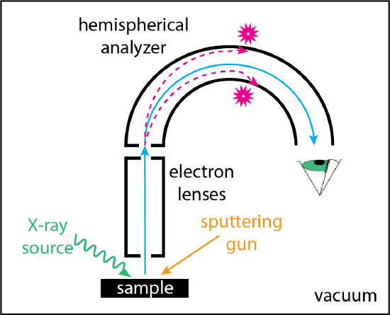
The instrumentation for AES can be coupled with an XPS spectrometer or be a stand-alone instrument. In either case, the basic instrumentation is similar to that shown in Figure \(\PageIndex{3}\), although AES spectra are usually initiated using an electron gun as a source instead of an X-ray source. One advantage to using an electron gun is that it can be focused into a smaller beam and can then easily rastered across a surface, allowing for imaging of the sample's surface. Depth profiling, using an ion beam to remove layers of the sample, is another common use of AES.

Figure \(\PageIndex{8}\) provides an example of a typical AES spectrum, in this case for the mineral calcite, CaCO₃. The raw data, on the left, shows the intensity of the signal as a count of electrons with a particular kinetic energy. The large background signal is from electrons that lose kinetic energy as the result of inelastic collisions. The two broad features between approximately 100 eV and 600 eV are the Auger peaks for calcium and for oxygen. The peaks in this case are easy to see because the two analytes are present in bulk. For a trace-level analyte, the Auger peaks in a normal plot may be difficult to see. For this reason, Auger spectra are usually presented by plotting the derivative of the raw data giving the spectrum on the right.

Figure \(\PageIndex{8}\): AES spectrum for the mineral calcite, CaCO₃. The figure on the left shows the spectrum as initially recorded and the figure on the right shows the data after taking the derivative of counts as a function of energy. The original data used to create thid figure is from the xpslibrary.

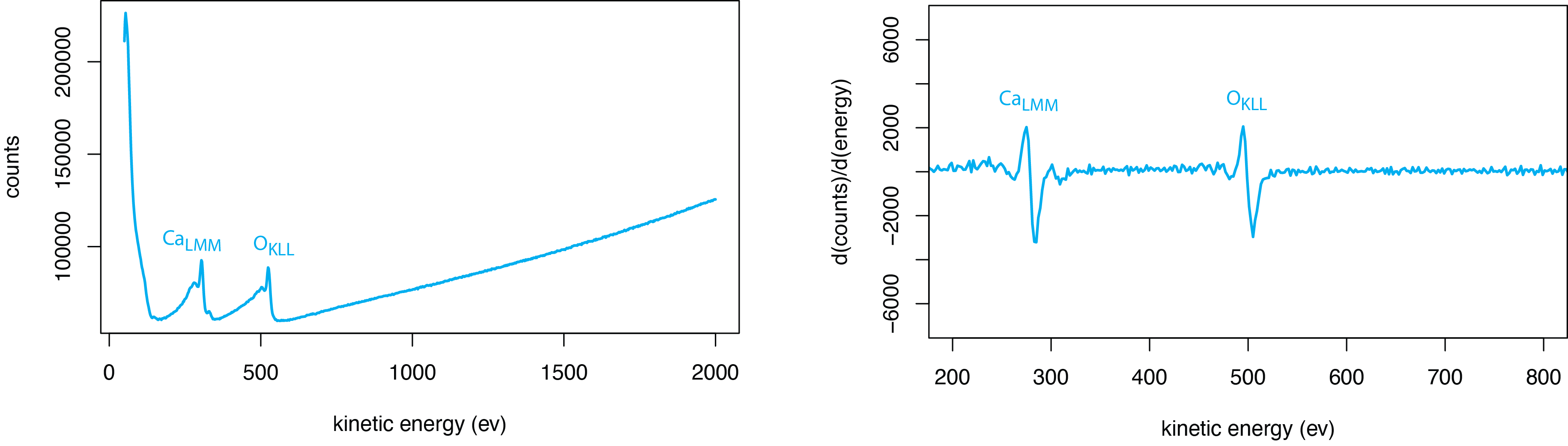
Figure \(\PageIndex{9}\) provides an example of how AES is used to study changes in the composition of a single crystal of CaCO₃ that was allowed to equilibrate with a solution containing Mg²⁺ ions. The sample was mounted on a sample probe and the AES spectrum recorded. An Ar⁺ ion beam was used to remove layers of the sample while the spectrometer was used to record spectra of the sample. As expected, the surface is enriched in Mg²⁺ ions that diffused into the crystal with the relative concentration of Mg²⁺ decreasing. The relative abundance of Ca²⁺ increases with depth; the relative concentration of oxygen remains more or less constant with depth.

Figure \(\PageIndex{9}\): Depth profiles for calcium, oxygen, and magnesium in a sample of CaCO₃ that was suspended in a solution of Mg2+ ion. The shading for each element shows the relative abundance of the element with depth. See Mucci, A.; Morse, J. W.; Kaminsky, M. S. "Auger Spectroscopy Analysis of Magnesian Calcite Overgrowths Precipitated From Seawater and Solutions of Similar Composition," Am. J. Sci. 1985, 289-305 for the paper suggesting this figure.

Secondary-Ion Mass Spectrometry (SIMS)

In SIMS we bombard the surface of a sample with an energetic primary beam—typically 5-20 keV—of an ion, such as Ar⁺, O₂⁺, or Cs⁺. The primary ion penetrates the sample's surface, ejecting a variety of particles, including neutral atoms, electrons, and, more importantly, secondary ions (singly-charged or multiply charged cations and anions, and clusters of ions). These secondary ions are characterized by their mass-to-charge ratios and by their kinetic energies. The use of a primary ion beam of Cs⁺ favors the formation of secondary ions that are anions, and a primary beam of O₂⁺ favors the formation of secondary ions that are cations.

The instrumentation for SIMS includes an ion gun for generating the primary beam and a mass spectrometer for analyzing the secondary ions. In static mode, the primary ion beam is run using a low current density that minimizes the extent to which the sample's outermost layers are removed. In dynamic mode, the primary beam is run at a higher current density that removes more of the sample's surface. Dynamic SIMS is well suited to depth profiling. High mass resolution is obtained using a time-of-flight mass analyzer or a double-focusing mass analyzer; see Chapter 20 for a discussion of different types of mass analyzers.

SIMS is well suited for imaging as the positively charged primary ion can be rastered across the sample's surface. Figure \(\PageIndex{10}\) provides an example of imaging a surface using SIMS by measuring the yield of ¹⁴N¹²C ions while rastering the primary ion beam across a 10 µm \(\times \) 10 µm section of the sample.

Figure \(\PageIndex{10}\): Image created using the R package lans2r ["lans2r: Work with Look at NanoSims Data in R", Sebastian Kopf, R package version 1.1.0, 2020]. The image shows the analysis of a 10 µm by 10 µm portion of a surface for the ¹⁴N¹²C ion, the two major isotopes of carbon and nitrogen. The bright areas have larger total ion counts.