19.3: NMR Spectrometers

Earlier in this chapter, we noted that there are two basic experimental designs for recording a NMR spectrum. One is a continuous-wave instrument in which the range of frequencies over which the nucleus of interest absorb is scanned linearly, exciting the different nuclei sequentially. Most instruments, however, use pulses of RF radiation to excite all nuclei at the same time and then use a Fourier transform to recover the signals from the individual nuclei. Our attention in this chapter is limited to instruments for FT-NMR.

Components of Fourier Transform Spectrometers

Figure \(\PageIndex{1}\) includes a photograph of 400 MHz NMR and a cut-away illustration of the instrument; together, these show the key components of a FT-NMR: a magnet that provides the applied magnetic field, \(B_0\), a nucleus-dependent probe that provides the radio-frequency signal that yields the magnetic field, \(B_1\), and a way to insert the sample into the instrument. The NMR in the photograph also is equipped with a sample changer that allows the user to load 30 or more samples that are analyzed sequentially.

Figure \(\PageIndex{1}\). Photograph of a 400 MHz NMR and an illustration of the magnet's housing and the location of the sample.

Magnets

The NMR in Figure \(\PageIndex{1}\) is described as having a frequency, \(\nu\), of 400 MHz. The relationship between frequency and the magnet's field strength, \(B_0\), is given by the equation

\[\nu = \frac{\gamma B_0}{2 \pi} \label{compent1} \]

where \(\gamma\) is the magnetogyric ratio for the nucleus. A NMR's frequency is defined in terms of a nucleus of ¹H; thus, a 400 MHz NMR has a magnet with a field strength of

\[B_0 = \frac{(2 \pi) \times \nu}{\gamma} = \frac{(2 \pi) \times (400 \times 10^6 \text{ s}^{-1})}{2.68 \times 10^{8} \text{ rad T}^{-1} \text{ s}^{-1}} = 9.4 \text{ T} \nonumber \]

Early instruments used a permanent magnet and were limited to field strengths of 0.7, 1.4, and 2.1 T, or 30, 60, and 90 MHz. As higher frequencies provide for greater sensitivity and resolution, modern instruments use a tightly wrapped coil of wire—typically a niobium/tin alloy or a niobium/titanium wire—that becomes superconducting when cooled to the temperature of liquid He (4.2 K). The result is a magnetic field strength of as much as 21 T or 900 MHz for ¹H NMR. The magnetic coil is held within a reservoir of liquid He, which, itself, is held within a reservoir of liquid N₂.

To be useful, the magnetic field must remain stable—that is, it must not drift—and it must be homogeneous throughout the sample. These are accomplished by using a reference to lock the magnetic field in place and by shimming.

Locking the Magnetic Field

Samples for NMR are prepared using a solvent in which the protons are replaced with deuterium. For example, instead of using chloroform, CHCl₃, as a solvent, we use deuterated chloroform, CDCl₃, where D is equivalent to ²H. This has the benefit of providing a solvent that will not contribute to the signals in the NMR spectrum. It also has the benefit that ²H has a spin of \(I = 1\), and a corresponding Larmor frequency. By monitoring the frequency at which ²H absorbs, the instrument can use a feed-back loop to maintain its value by adjusting the magnet's field strength.

Shimming

A magnetic field that is not homogeneous is like a table with four legs, one of which is just a bit shorter than the others. To balance the table, we place a small wedge, or shim, under the shorter leg. When a magnetic field is not homogeneous, small, localized adjustments are made to the magnetic field using a set of shimming coils arranged around the sample. Shimming can be accomplished by the operator by monitoring the quality of the signal for a particular nucleus, however, most instruments use an algorithm that allows the instrument to shim itself.

The Sample Inlet and the Sample Probe

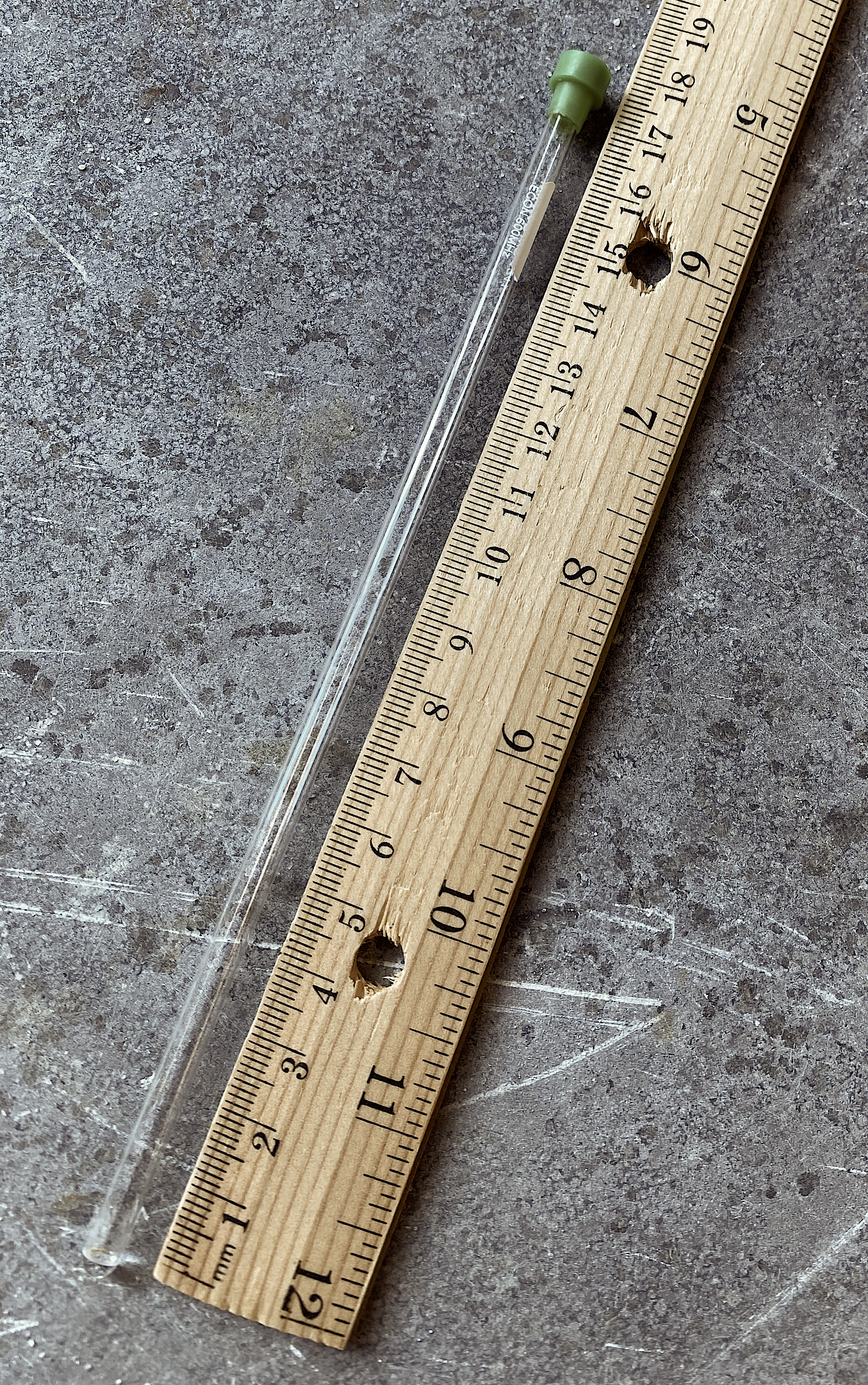
The center of the instrument, which runs from the sample input at the top to the sample probe at the bottom, is open to the laboratory environment and is at room temperature. The sample is placed in a cylindrical tube (Figure \(\PageIndex{2}a\)), that is made from thin-walled borosilicate glass and is 180 mm long and 5 mm in diameter. The tube is then inserted into a teflon sleeve—called a spinner—as shown in Figure \(\PageIndex{2}b\), which is designed to both situate the sample at the proper depth within the sample probe, and to spin the sample about its long axis. This spinning is used to ensure that the sample averages out any inhomogeneities in the magnetic field not resovled by shimming.

Figure \(\PageIndex{2}\). Photographs showing an NMR sample tube (left) and the spinner assembly (right).

The sample probe contains the coils needed to excite the sample and to detect the NMR signal as the excited states undergo relaxation. Figure \(\PageIndex{3}\) shows two configurations for this; in both configurations, the same coil is used for both excitation and detection. In the design on the left, which uses a permanent magnet, the applied magnetic field, \(B_0\), is oriented horizontally across the sample's diameter and the radio frequency electromagnetic radiation and its field, \(B_1\) is oriented vertically using a spiral coil. In the design on the right, which is used with a superconducting magnet, the applied magnetic field, \(B_0\), is oriented vertically and the pulse of radio frequency electromagnetic radiation and its field, \(B_1\), is oriented horizontally using a saddle coil.

Figure \(\PageIndex{3}\). Two configurations for applying the magnetic fields \(B_0\) and \(B_1\). The configuration on the left is used with a permanent, such as a continuous wave instrument or a benchtop FT-NMR. The configuration on the right is used with a superconducting magnet, such as the instrument in Figure \(\PageIndex{1}\).

Data Processing

In Chapter 19.1 we used the following figure to describe a pulse NMR experiment. Following a pulse that is applied for 1–10 µs, the free-induction decay, FID, is recorded for a period of time that may range from as little as 0.1 seconds to as long as 10 seconds, depending on the nucleus being probed.

Figure \(\PageIndex{4}\). An example of a pulse sequence for FT-NMR. See the text for a description of the terms shown here.

The FID is an analog signal in the form of a voltage, typically in the µV range. This analog signal must be converted into a digital signal for data processing, which is called an analog-to-digital conversion, ADC. Two important considerations are needed here: how to ensure that the signal—more specifically, the location of the peaks in the NMR spectrum—is not distorted, and how to accomplish the ADC when the frequencies are on the order of hundreds of MHz.

Analog-to-Digital Conversion

An analog-to-digital converter maps the signal onto a limited number of possible values—expressed in binary notation—and are characterized by the number of available bits. A 2-bit ADC convertor, for example, is limited to \(2^2 = 4\) possible binary values of 00, 01, 10, and 11 that correspond to the decimal numbers 1, 2, 3, and 4. Having only four possible values, of course, would distort the FID pattern in Figure \(\PageIndex{4}\) from a smoothly varying oscillating signal into a series of steps. Using an ADC convertor with 16 bits allows for 65,536 unique digital values, a significant improvement. Another form of distortion occurs if we do not sample the FID with sufficient frequency. Consider, for example, the simple sine wave in Figure \(\PageIndex{5}a\) that is shown as a solid line. If we sample this signal only five times over a period of less than four complete cycles, as shown by the five equally-spaced dots in Figure \(\PageIndex{5}a\), then the apparent signal is that shown by the dadshed line.

Figure \(\PageIndex{5}\): Effect of sampling frequency when monitoring a periodic signal. Individual samples are shown by the red dots (•). In (a) the sampling frequency is approximately 1.5 samples per period. The dashed red line shows the apparent signal based on five samples and the solid blue line shows the true signal. In (b) a sampling frequency of six samples per period accurately reproduces the true signal.

According to the Nyquist theorem, to determine accurately the frequency of a periodic signal, we must sample the signal at least twice during each cycle or period. Given a sampling rate of \(\Delta\), the following equation

\[\Delta = \frac{1}{2 \nu_\text{max}} \label{adc1} \]

defines the highest frequency, \(\nu_\text{max}\), that we can monitor accurately. A sampling rate of six samples per period is more than sufficient to reproduce the real signal in Figure \(\PageIndex{5}\).

A peak with a frequency that is greater than \(\nu_\text{max}\) is not absent from the spectrum; instead, it simply appears at a different location. For example, suppose we can monitor accurately any frequency within the window shown in Figure \(\PageIndex{6}\) and that we only measure frequencies within this window. A peak with a frequency that is greater than what we can measure accurately by \(\Delta \nu\) appears at an apparent frequency that is \(\Delta \nu\) greater than the frequency window's lower limit. This is called folding.

Figure \(\PageIndex{6}\). Illustration showing the origin of folding in which a peak in the NMR spectrum appears at a value of \(\delta\) that is different from its actual value.

Managing MHz Signals

The instrument in Figure \(\PageIndex{1}\) is a 400 MHz NMR. This is a range of frequencies that is too large for an analog-to-digital convertor to handle with accuracy. The frequency window of interest to us, however, is typically 10 ppm for ¹H NMR (see Chapter 19.2 to review the NMR scale). For a 400 MHz NMR this corresponds to just 4000 Hz, with the useful range running from 400.000 MHz to 400.004 MHz. Subtracting the instrument's frequency of 400 MHz from the signal's frequency limits the latter to the range of 0–4000 Hz, a range that is easy for an ADC to handle.

Signal Integrators

Integrating to determine the area under the peaks provides a way to gain some quantitative information about the sample. Figure \(\PageIndex{7}\) shows the integration of the NMR of propane first seen in Chapter 19.2. Integration of the peak for the two methyl groups gives a result of 1766 and integration of the peak for the methylene group gives a result of 710. The ratio of the two is

\[\frac{1766}{710} = 2.5 \nonumber \]

which is somewhat smaller than the expected 3:1 ratio.

Figure \(\PageIndex{1}\). Illustration of integration. The original data used to construct this spectrum is here and was obtained on a 300 MHz instrument.