15.5: Evaluation of Molecular Luminescence

Last updated
Save as PDF

Page ID: 366539

$ \newcommand{\vecs}[1]{\overset { \scriptstyle \rightharpoonup} {\mathbf{#1}} } $

$ \newcommand{\vecd}[1]{\overset{-\!-\!\rightharpoonup}{\vphantom{a}\smash {#1}}} $

$ \newcommand{\id}{\mathrm{id}}$ $ \newcommand{\Span}{\mathrm{span}}$

( \newcommand{\kernel}{\mathrm{null}\,}\) $ \newcommand{\range}{\mathrm{range}\,}$

$ \newcommand{\RealPart}{\mathrm{Re}}$ $ \newcommand{\ImaginaryPart}{\mathrm{Im}}$

$ \newcommand{\Argument}{\mathrm{Arg}}$ $ \newcommand{\norm}[1]{\| #1 \|}$

$ \newcommand{\inner}[2]{\langle #1, #2 \rangle}$

$ \newcommand{\Span}{\mathrm{span}}$

$ \newcommand{\id}{\mathrm{id}}$

$ \newcommand{\Span}{\mathrm{span}}$

$ \newcommand{\kernel}{\mathrm{null}\,}$

$ \newcommand{\range}{\mathrm{range}\,}$

$ \newcommand{\RealPart}{\mathrm{Re}}$

$ \newcommand{\ImaginaryPart}{\mathrm{Im}}$

$ \newcommand{\Argument}{\mathrm{Arg}}$

$ \newcommand{\norm}[1]{\| #1 \|}$

$ \newcommand{\inner}[2]{\langle #1, #2 \rangle}$

$ \newcommand{\Span}{\mathrm{span}}$ $ \newcommand{\AA}{\unicode[.8,0]{x212B}}$

$ \newcommand{\vectorA}[1]{\vec{#1}} % arrow$

$ \newcommand{\vectorAt}[1]{\vec{\text{#1}}} % arrow$

$ \newcommand{\vectorB}[1]{\overset { \scriptstyle \rightharpoonup} {\mathbf{#1}} } $

$ \newcommand{\vectorC}[1]{\textbf{#1}} $

$ \newcommand{\vectorD}[1]{\overrightarrow{#1}} $

$ \newcommand{\vectorDt}[1]{\overrightarrow{\text{#1}}} $

$ \newcommand{\vectE}[1]{\overset{-\!-\!\rightharpoonup}{\vphantom{a}\smash{\mathbf {#1}}}} $

$ \newcommand{\vecs}[1]{\overset { \scriptstyle \rightharpoonup} {\mathbf{#1}} } $

$ \newcommand{\vecd}[1]{\overset{-\!-\!\rightharpoonup}{\vphantom{a}\smash {#1}}} $

$\newcommand{\avec}{\mathbf a}$ $\newcommand{\bvec}{\mathbf b}$ $\newcommand{\cvec}{\mathbf c}$ $\newcommand{\dvec}{\mathbf d}$ $\newcommand{\dtil}{\widetilde{\mathbf d}}$ $\newcommand{\evec}{\mathbf e}$ $\newcommand{\fvec}{\mathbf f}$ $\newcommand{\nvec}{\mathbf n}$ $\newcommand{\pvec}{\mathbf p}$ $\newcommand{\qvec}{\mathbf q}$ $\newcommand{\svec}{\mathbf s}$ $\newcommand{\tvec}{\mathbf t}$ $\newcommand{\uvec}{\mathbf u}$ $\newcommand{\vvec}{\mathbf v}$ $\newcommand{\wvec}{\mathbf w}$ $\newcommand{\xvec}{\mathbf x}$ $\newcommand{\yvec}{\mathbf y}$ $\newcommand{\zvec}{\mathbf z}$ $\newcommand{\rvec}{\mathbf r}$ $\newcommand{\mvec}{\mathbf m}$ $\newcommand{\zerovec}{\mathbf 0}$ $\newcommand{\onevec}{\mathbf 1}$ $\newcommand{\real}{\mathbb R}$ $\newcommand{\twovec}[2]{\left[\begin{array}{r}#1 \\ #2 \end{array}\right]}$ $\newcommand{\ctwovec}[2]{\left[\begin{array}{c}#1 \\ #2 \end{array}\right]}$ $\newcommand{\threevec}[3]{\left[\begin{array}{r}#1 \\ #2 \\ #3 \end{array}\right]}$ $\newcommand{\cthreevec}[3]{\left[\begin{array}{c}#1 \\ #2 \\ #3 \end{array}\right]}$ $\newcommand{\fourvec}[4]{\left[\begin{array}{r}#1 \\ #2 \\ #3 \\ #4 \end{array}\right]}$ $\newcommand{\cfourvec}[4]{\left[\begin{array}{c}#1 \\ #2 \\ #3 \\ #4 \end{array}\right]}$ $\newcommand{\fivevec}[5]{\left[\begin{array}{r}#1 \\ #2 \\ #3 \\ #4 \\ #5 \\ \end{array}\right]}$ $\newcommand{\cfivevec}[5]{\left[\begin{array}{c}#1 \\ #2 \\ #3 \\ #4 \\ #5 \\ \end{array}\right]}$ $\newcommand{\mattwo}[4]{\left[\begin{array}{rr}#1 \amp #2 \\ #3 \amp #4 \\ \end{array}\right]}$ $\newcommand{\laspan}[1]{\text{Span}\{#1\}}$ $\newcommand{\bcal}{\cal B}$ $\newcommand{\ccal}{\cal C}$ $\newcommand{\scal}{\cal S}$ $\newcommand{\wcal}{\cal W}$ $\newcommand{\ecal}{\cal E}$ $\newcommand{\coords}[2]{\left\{#1\right\}_{#2}}$ $\newcommand{\gray}[1]{\color{gray}{#1}}$ $\newcommand{\lgray}[1]{\color{lightgray}{#1}}$ $\newcommand{\rank}{\operatorname{rank}}$ $\newcommand{\row}{\text{Row}}$ $\newcommand{\col}{\text{Col}}$ $\renewcommand{\row}{\text{Row}}$ $\newcommand{\nul}{\text{Nul}}$ $\newcommand{\var}{\text{Var}}$ $\newcommand{\corr}{\text{corr}}$ $\newcommand{\len}[1]{\left|#1\right|}$ $\newcommand{\bbar}{\overline{\bvec}}$ $\newcommand{\bhat}{\widehat{\bvec}}$ $\newcommand{\bperp}{\bvec^\perp}$ $\newcommand{\xhat}{\widehat{\xvec}}$ $\newcommand{\vhat}{\widehat{\vvec}}$ $\newcommand{\uhat}{\widehat{\uvec}}$ $\newcommand{\what}{\widehat{\wvec}}$ $\newcommand{\Sighat}{\widehat{\Sigma}}$ $\newcommand{\lt}{<}$ $\newcommand{\gt}{>}$ $\newcommand{\amp}{&}$ $\definecolor{fillinmathshade}{gray}{0.9}$

Scale of Operation

Photoluminescence spectroscopy is used for the routine analysis of trace and ultratrace analytes in macro and meso samples. Detection limits for fluorescence spectroscopy are influenced by the analyte’s quantum yield. For an analyte with $\Phi_f > 0.5$, a picomolar detection limit is possible when using a high quality spectrofluorometer. For example, the detection limit for quinine sulfate, for which $\Phi$ is 0.55, generally is between 1 part per billion and 1 part per trillion. Detection limits for phosphorescence are somewhat higher, with typical values in the nanomolar range for low-temperature phosphorimetry and in the micromolar range for room-temperature phosphorimetry using a solid substrate.

Accuracy

The accuracy of a fluorescence method generally is between 1–5% when spectral and chemical interferences are insignificant. Accuracy is limited by the same types of problems that affect other optical spectroscopic methods. In addition, accuracy is affected by interferences that affect the fluorescent quantum yield. The accuracy of phosphorescence is somewhat greater than that for fluorescence.

Precision

The relative standard deviation for fluorescence usually is between 0.5–2% when the analyte’s concentration is well above its detection limit. Precision usually is limited by the stability of the excitation source. The precision for phosphorescence often is limited by reproducibility in preparing samples for analysis, with relative standard deviations of 5–10% being common.

Sensitivity

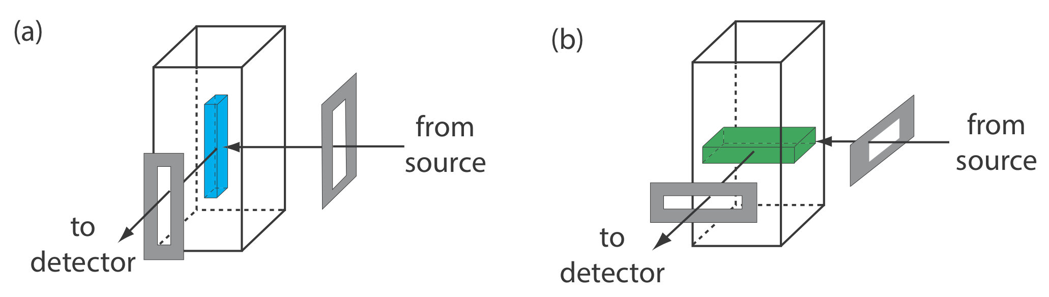
The sensitivity of a fluorescent or a phosphorescent method is affected by a number of parameters. We already have considered the importance of quantum yield and the effect of temperature and solution composition on $\Phi_f$ and $\Phi_p$. Besides quantum yield, sensitivity is improved by using an excitation source that has a greater emission intensity, P₀, at the desired wavelength, and by selecting an excitation wavelength for which the analyte has a greater molar absorptivity, $\varepsilon$. Another approach for improving sensitivity is to increase the volume from which emission is monitored. Figure $\PageIndex{1}$ shows how rotating a monochromator’s slits from their usual vertical orientation to a horizontal orientation increases the sampling volume. The result can increase the emission from the sample by $5-30 \times$.

Use of slit orientation to change the volume from which fluorescence is measured. — Figure $\PageIndex{1}$. Use of slit orientation to change the volume from which fluorescence is measured: (a) vertical slit orientation; (b) horizontal slit orientation. Suppose the slit’s dimensions are 0.1 mm $\times$ 3 mm. In (a) the dimensions of the sampling volume are 0.1 mm $\times$ 0.1 mm $\times$ 3 mm, or 0.03 mm³. For (b) the dimensions of the sampling volume are 0.1 mm $\times$ 3 mm $\times$ 3 mm, or 0.9 mm³, a 30-fold increase in the sampling volume.

Selectivity

The selectivity of fluorescence and phosphorescence is superior to that of absorption spectrophotometry for two reasons: first, not every compound that absorbs radiation is fluorescent or phosphorescent; and, second, selectivity between an analyte and an interferent is possible if there is a difference in either their excitation or their emission spectra. The total emission intensity is a linear sum of that from each fluorescent or phosphorescent species. The analysis of a sample that contains n analytes, therefore, is accomplished by measuring the total emission intensity at n wavelengths.

Time, Cost, and Equipment

As with other optical spectroscopic methods, fluorescent and phosphorescent methods provide a rapid means for analyzing samples and are capable of automation. Fluorometers are relatively inexpensive, ranging from several hundred to several thousand dollars, and often are satisfactory for quantitative work. Spectrofluorometers are more expensive, with models often exceeding $50,000.

Search

Text Color

Text Size

Margin Size

Font Type