15.3: Applications and Photoluminescence methods

Quantitative Applications

Molecular fluorescence and, to a lesser extent, phosphorescence are used for the direct or indirect quantitative analysis of analytes in a variety of matrices. A direct quantitative analysis is possible when the analyte’s fluorescent or phosphorescent quantum yield is favorable. If the analyte is not fluorescent or phosphorescent, or if the quantum yield is unfavorable, then an indirect analysis may be feasible. One approach is to react the analyte with a reagent to form a product that is fluorescent or phosphorescent. Another approach is to measure a decrease in fluorescence or phosphorescence when the analyte is added to a solution that contains a fluorescent or phosphorescent probe molecule. A decrease in emission is observed when the reaction between the analyte and the probe molecule enhances radiationless deactivation or results in a nonemitting product. The application of fluorescence and phosphorescence to inorganic and organic analytes are considered in this section.

Inorganic Analytes

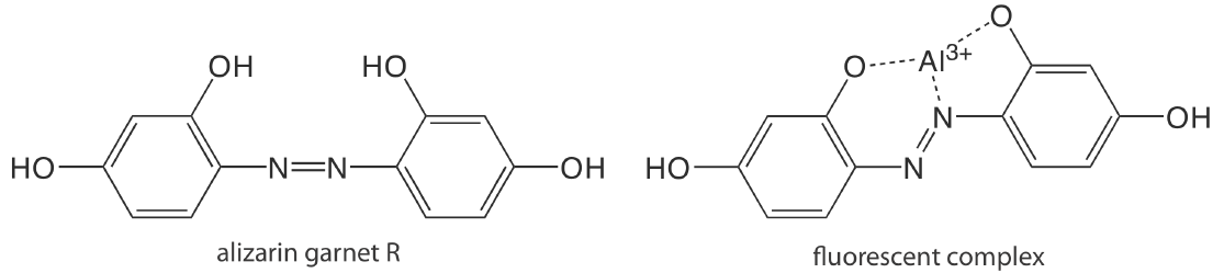
Except for a few metal ions, most notably \(\text{UO}_2^+\), most inorganic ions are not sufficiently fluorescent for a direct analysis. Many metal ions are determined indirectly by reacting with an organic ligand to form a fluorescent or, less commonly, a phosphorescent metal–ligand complex. One example is the reaction of Al³⁺ with the sodium salt of 2, 4, 3′-trihydroxyazobenzene-5′-sulfonic acid—also known as alizarin garnet R—which forms a fluorescent metal–ligand complex (Figure \(\PageIndex{1}\)). The analysis is carried out using an excitation wavelength of 470 nm, with fluorescence monitored at 500 nm. Table \(\PageIndex{1}\) provides additional examples of chelating reagents that form fluorescent metal–ligand complexes with metal ions. A few inorganic nonmetals are determined by their ability to decrease, or quench, the fluorescence of another species. One example is the analysis for F^– based on its ability to quench the fluorescence of the Al³⁺–alizarin garnet R complex.

Figure \(\PageIndex{1}\). Structure of alizarin garnet R and its metal–ligand complex with Al³⁺.

Table \(\PageIndex{1}\). Chelating Agents for the Fluorescent Analysis of Metal Ions

chelating agent	metal ions
8-hydroxyquinoline	Al^3^+, Be^2^+, Zn^2^+, Li^+, Mg^2^+ (and others)
flavonal	Zr^2^+, Sn^4^+
benzoin	\(\text{B}_4\text{O}_6^{2-}\), Zn^2^+
\(2^{\prime},3^{\prime},4^{\prime},5,7-\text{pentahydroxylflavone}\)	Be^2^+
2-(o-hydroxyphenyl) benzoxazole	Cd^2^+

Organic Analytes

As noted earlier, organic compounds that contain aromatic rings generally are fluorescent and aromatic heterocycles often are phosphorescent. Table \(\PageIndex{2}\) provides examples of several important biochemical, pharmaceutical, and environmental compounds that are analyzed quantitatively by fluorimetry or phosphorimetry. If an organic analyte is not naturally fluorescent or phosphorescent, it may be possible to incorporate it into a chemical reaction that produces a fluorescent or phosphorescent product. For example, the enzyme creatine phosphokinase is determined by using it to catalyze the formation of creatine from phosphocreatine. Reacting the creatine with ninhydrin produces a fluorescent product of unknown structure.

Table \(\PageIndex{2}\). Examples of Naturally Photoluminescent Organic Analytes

class	compounds (F = fluorescence, P = phosphorescence)
aromatic amino acids	phenylalanine (F) tyrosine (F) tryptophan (F, P)
vitamins	vitamin A (F) vitamin B2 (F) vitamin B6 (F) vitamin B12 (F) vitamin E (F) folic acid (F)
catecholamines	dopamine (F) norepinephrine (F)
pharmaceuticals and drugs	quinine (F) salicylic acid (F, P) morphine (F) barbiturates (F) LSD (F) codeine (P) caffeine (P) sulfanilamide (P)
environmental pollutants	pyrene (F) benzo[a]pyrene (F) organothiophosphorous pesticides (F) carbamate insecticides (F) DDT (P)

Standardizing the Method

In Section 15.1 we showed that the intensity of fluorescence or phosphorescence is a linear function of the analyte’s concentration provided that the sample’s absorbance of source radiation (\(A = \varepsilon bC\)) is less than approximately 0.01. Calibration curves often are linear over four to six orders of magnitude for fluorescence and over two to four orders of magnitude for phosphorescence. For higher concentrations of analyte the calibration curve becomes nonlinear because the assumption that absorbance is negligible no longer apply. Nonlinearity may be observed for smaller concentrations of analyte fluorescent or phosphorescent contaminants are present. As discussed earlier, quantum efficiency is sensitive to temperature and sample matrix, both of which must be controlled when using external standards. In addition, emission intensity depends on the molar absorptivity of the photoluminescent species, which is sensitive to the sample matrix.

Representative Method: Determination of Quinine in Urine

The best way to appreciate the theoretical and the practical details discussed in this section is to carefully examine a typical analytical method. Although each method is unique, the following description of the determination of quinine in urine provides an instructive example of a typical procedure. The description here is based on Mule, S. J.; Hushin, P. L. Anal. Chem. 1971, 43, 708–711, and O’Reilly, J. E.; J. Chem. Educ. 1975, 52, 610–612.

Description of the Method

Quinine is an alkaloid used to treat malaria. It is a strongly fluorescent compound in dilute solutions of H₂SO₄ (\(\Phi_f = 0.55\)). Quinine’s excitation spectrum has absorption bands at 250 nm and 350 nm and its emission spectrum has a single emission band at 450 nm. Quinine is excreted rapidly from the body in urine and is determined by measuring its fluorescence following its extraction from the urine sample.

Procedure

Transfer a 2.00-mL sample of urine to a 15-mL test tube and use 3.7 M NaOH to adjust its pH to between 9 and 10. Add 4 mL of a 3:1 (v/v) mixture of chloroform and isopropanol and shake the contents of the test tube for one minute. Allow the organic and the aqueous (urine) layers to separate and transfer the organic phase to a clean test tube. Add 2.00 mL of 0.05 M H₂SO₄ to the organic phase and shake the contents for one minute. Allow the organic and the aqueous layers to separate and transfer the aqueous phase to the sample cell. Measure the fluorescent emission at 450 nm using an excitation wavelength of 350 nm. Determine the concentration of quinine in the urine sample using a set of external standards in 0.05 M H₂SO₄, prepared from a 100.0 ppm solution of quinine in 0.05 M H₂SO₄. Use distilled water as a blank.

Questions

1. Chloride ion quenches the intensity of quinine’s fluorescent emission. For example, in the presence of 100 ppm NaCl (61 ppm Cl^–) quinine’s emission intensity is only 83% of its emission intensity in the absence of chloride. The presence of 1000 ppm NaCl (610 ppm Cl^–) further reduces quinine’s fluorescent emission to less than 30% of its emission intensity in the absence of chloride. The concentration of chloride in urine typically ranges from 4600–6700 ppm Cl^–. Explain how this procedure prevents an interference from chloride.

The procedure uses two extractions. In the first of these extractions, quinine is separated from urine by extracting it into a mixture of chloroform and isopropanol, leaving the chloride ion behind in the original sample.

2. Samples of urine may contain small amounts of other fluorescent compounds, which will interfere with the analysis if they are carried through the two extractions. Explain how you can modify the procedure to take this into account?

One approach is to prepare a blank that uses a sample of urine known to be free of quinine. Subtracting the blank’s fluorescent signal from the measured fluorescence from urine samples corrects for the interfering compounds.

3. The fluorescent emission for quinine at 450 nm can be induced using an excitation frequency of either 250 nm or 350 nm. The fluorescent quantum efficiency is the same for either excitation wavelength. Quinine’s absorption spectrum shows that \(\varepsilon_{250}\) is greater than \(\varepsilon_{350}\). Given that quinine has a stronger absorbance at 250 nm, explain why its fluorescent emission intensity is greater when using 350 nm as the excitation wavelength.

We know that I_f is a function of the following terms: k, \(\Phi_f\), P₀, \(\varepsilon\), b, and C. We know that \(\Phi_f\), b, and C are the same for both excitation wavelengths and that \(\varepsilon\) is larger for a wavelength of 250 nm; we can, therefore, ignore these terms. The greater emission intensity when using an excitation wavelength of 350 nm must be due to a larger value for P₀ or k . In fact, P₀ at 350 nm for a high-pressure Xe arc lamp is about 170% of that at 250 nm. In addition, the sensitivity of a typical photomultiplier detector (which contributes to the value of k) at 350 nm is about 140% of that at 250 nm.

Example \(\PageIndex{1}\)

To evaluate the method described iabove, a series of external standard are prepared and analyzed, providing the results shown in the following table. All fluorescent intensities are corrected using a blank prepared from a quinine-free sample of urine. The fluorescent intensities are normalized by setting I_f for the highest concentration standard to 100.

[quinine] (µg/mL)	If
1.00	10.11
3.00	30.20
5.00	49.84
7.00	69.89
10.00	100.0

After ingesting 10.0 mg of quinine, a volunteer provides a urine sample 24-h later. Analysis of the urine sample gives a relative emission intensity of 28.16. Report the concentration of quinine in the sample in mg/L and the percent recovery for the ingested quinine.

Solution

Linear regression of the relative emission intensity versus the concentration of quinine in the standards gives the calibration curve shown below and the following calibration equation.

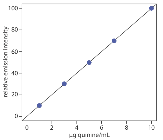
\[I_{f}=0.122+9.978 \times \frac{\mathrm{g} \text { quinine }}{\mathrm{mL}} \nonumber \]

Substituting the sample’s relative emission intensity into the calibration equation gives the concentration of quinine as 2.81 μg/mL. Because the volume of urine taken, 2.00 mL, is the same as the volume of 0.05 M H₂SO₄ used to extract the quinine, the concentration of quinine in the urine also is 2.81 μg/mL. The recovery of the ingested quinine is

\[\frac{\frac{2.81 \ \mu \mathrm{g} \text { quinine }}{\mathrm{mL} \text { urine }} \times 2.00 \ \mathrm{mL} \text { urine } \times \frac{1 \mathrm{mg}}{1000 \ \mu \mathrm{g}}} {10.0 \ \mathrm{mg} \text { quinine ingested }} \times 100=0.0562 \% \nonumber \]

It can take 10–11 days for the body to completely excrete quinine so it is not surprising that such a small amount of quinine is recovered from this sample of urine.