15.1: Theory of Fluorescence and Phosphorescence
- Page ID
- 366514

\( \newcommand{\vecs}[1]{\overset { \scriptstyle \rightharpoonup} {\mathbf{#1}} } \)
\( \newcommand{\vecd}[1]{\overset{-\!-\!\rightharpoonup}{\vphantom{a}\smash {#1}}} \)
\( \newcommand{\id}{\mathrm{id}}\) \( \newcommand{\Span}{\mathrm{span}}\)
( \newcommand{\kernel}{\mathrm{null}\,}\) \( \newcommand{\range}{\mathrm{range}\,}\)
\( \newcommand{\RealPart}{\mathrm{Re}}\) \( \newcommand{\ImaginaryPart}{\mathrm{Im}}\)
\( \newcommand{\Argument}{\mathrm{Arg}}\) \( \newcommand{\norm}[1]{\| #1 \|}\)
\( \newcommand{\inner}[2]{\langle #1, #2 \rangle}\)
\( \newcommand{\Span}{\mathrm{span}}\)
\( \newcommand{\id}{\mathrm{id}}\)
\( \newcommand{\Span}{\mathrm{span}}\)
\( \newcommand{\kernel}{\mathrm{null}\,}\)
\( \newcommand{\range}{\mathrm{range}\,}\)
\( \newcommand{\RealPart}{\mathrm{Re}}\)
\( \newcommand{\ImaginaryPart}{\mathrm{Im}}\)
\( \newcommand{\Argument}{\mathrm{Arg}}\)
\( \newcommand{\norm}[1]{\| #1 \|}\)
\( \newcommand{\inner}[2]{\langle #1, #2 \rangle}\)
\( \newcommand{\Span}{\mathrm{span}}\) \( \newcommand{\AA}{\unicode[.8,0]{x212B}}\)
\( \newcommand{\vectorA}[1]{\vec{#1}} % arrow\)
\( \newcommand{\vectorAt}[1]{\vec{\text{#1}}} % arrow\)
\( \newcommand{\vectorB}[1]{\overset { \scriptstyle \rightharpoonup} {\mathbf{#1}} } \)
\( \newcommand{\vectorC}[1]{\textbf{#1}} \)
\( \newcommand{\vectorD}[1]{\overrightarrow{#1}} \)
\( \newcommand{\vectorDt}[1]{\overrightarrow{\text{#1}}} \)
\( \newcommand{\vectE}[1]{\overset{-\!-\!\rightharpoonup}{\vphantom{a}\smash{\mathbf {#1}}}} \)
\( \newcommand{\vecs}[1]{\overset { \scriptstyle \rightharpoonup} {\mathbf{#1}} } \)
\( \newcommand{\vecd}[1]{\overset{-\!-\!\rightharpoonup}{\vphantom{a}\smash {#1}}} \)
\(\newcommand{\avec}{\mathbf a}\) \(\newcommand{\bvec}{\mathbf b}\) \(\newcommand{\cvec}{\mathbf c}\) \(\newcommand{\dvec}{\mathbf d}\) \(\newcommand{\dtil}{\widetilde{\mathbf d}}\) \(\newcommand{\evec}{\mathbf e}\) \(\newcommand{\fvec}{\mathbf f}\) \(\newcommand{\nvec}{\mathbf n}\) \(\newcommand{\pvec}{\mathbf p}\) \(\newcommand{\qvec}{\mathbf q}\) \(\newcommand{\svec}{\mathbf s}\) \(\newcommand{\tvec}{\mathbf t}\) \(\newcommand{\uvec}{\mathbf u}\) \(\newcommand{\vvec}{\mathbf v}\) \(\newcommand{\wvec}{\mathbf w}\) \(\newcommand{\xvec}{\mathbf x}\) \(\newcommand{\yvec}{\mathbf y}\) \(\newcommand{\zvec}{\mathbf z}\) \(\newcommand{\rvec}{\mathbf r}\) \(\newcommand{\mvec}{\mathbf m}\) \(\newcommand{\zerovec}{\mathbf 0}\) \(\newcommand{\onevec}{\mathbf 1}\) \(\newcommand{\real}{\mathbb R}\) \(\newcommand{\twovec}[2]{\left[\begin{array}{r}#1 \\ #2 \end{array}\right]}\) \(\newcommand{\ctwovec}[2]{\left[\begin{array}{c}#1 \\ #2 \end{array}\right]}\) \(\newcommand{\threevec}[3]{\left[\begin{array}{r}#1 \\ #2 \\ #3 \end{array}\right]}\) \(\newcommand{\cthreevec}[3]{\left[\begin{array}{c}#1 \\ #2 \\ #3 \end{array}\right]}\) \(\newcommand{\fourvec}[4]{\left[\begin{array}{r}#1 \\ #2 \\ #3 \\ #4 \end{array}\right]}\) \(\newcommand{\cfourvec}[4]{\left[\begin{array}{c}#1 \\ #2 \\ #3 \\ #4 \end{array}\right]}\) \(\newcommand{\fivevec}[5]{\left[\begin{array}{r}#1 \\ #2 \\ #3 \\ #4 \\ #5 \\ \end{array}\right]}\) \(\newcommand{\cfivevec}[5]{\left[\begin{array}{c}#1 \\ #2 \\ #3 \\ #4 \\ #5 \\ \end{array}\right]}\) \(\newcommand{\mattwo}[4]{\left[\begin{array}{rr}#1 \amp #2 \\ #3 \amp #4 \\ \end{array}\right]}\) \(\newcommand{\laspan}[1]{\text{Span}\{#1\}}\) \(\newcommand{\bcal}{\cal B}\) \(\newcommand{\ccal}{\cal C}\) \(\newcommand{\scal}{\cal S}\) \(\newcommand{\wcal}{\cal W}\) \(\newcommand{\ecal}{\cal E}\) \(\newcommand{\coords}[2]{\left\{#1\right\}_{#2}}\) \(\newcommand{\gray}[1]{\color{gray}{#1}}\) \(\newcommand{\lgray}[1]{\color{lightgray}{#1}}\) \(\newcommand{\rank}{\operatorname{rank}}\) \(\newcommand{\row}{\text{Row}}\) \(\newcommand{\col}{\text{Col}}\) \(\renewcommand{\row}{\text{Row}}\) \(\newcommand{\nul}{\text{Nul}}\) \(\newcommand{\var}{\text{Var}}\) \(\newcommand{\corr}{\text{corr}}\) \(\newcommand{\len}[1]{\left|#1\right|}\) \(\newcommand{\bbar}{\overline{\bvec}}\) \(\newcommand{\bhat}{\widehat{\bvec}}\) \(\newcommand{\bperp}{\bvec^\perp}\) \(\newcommand{\xhat}{\widehat{\xvec}}\) \(\newcommand{\vhat}{\widehat{\vvec}}\) \(\newcommand{\uhat}{\widehat{\uvec}}\) \(\newcommand{\what}{\widehat{\wvec}}\) \(\newcommand{\Sighat}{\widehat{\Sigma}}\) \(\newcommand{\lt}{<}\) \(\newcommand{\gt}{>}\) \(\newcommand{\amp}{&}\) \(\definecolor{fillinmathshade}{gray}{0.9}\)The use of molecular fluorescence for qualitative analysis and for semi-quantitative analysis dates to the early to mid 1800s, with more accurate quantitative methods appearing in the 1920s. Instrumentation for fluorescence spectroscopy using a filter or a monochromator for wavelength selection appeared in, respectively, the 1930s and 1950s. Although the discovery of phosphorescence preceded that of fluorescence by almost 200 years, qualitative and quantitative applications of molecular phosphorescence did not receive much attention until after the development of fluorescence instrumentation.
Source of Fluorescence and Phosphorescence
Photoluminescence is divided into two categories: fluorescence and phosphorescence. A pair of electrons that occupy the same electronic ground state have opposite spins and are in a singlet spin state (Figure \(\PageIndex{1}a\)).
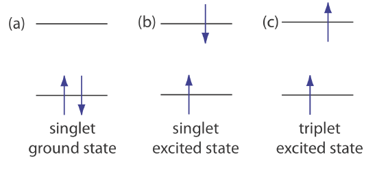
When an analyte absorbs an ultraviolet or a visible photon, one of its valence electrons moves from the ground state to an excited state with a conservation of the electron’s spin (Figure \(\PageIndex{1}b\)). Emission of a photon from a singlet excited state to the singlet ground state—or between any two energy levels with the same spin—is called fluorescence. The probability of fluorescence is very high and the average lifetime of an electron in the excited state is only 10–5–10–8 s. Fluorescence, therefore, rapidly decays once the source of excitation is removed.
In some cases an electron in a singlet excited state is transformed to a triplet excited state (Figure \(\PageIndex{1}c\)) in which its spin no is longer paired with the ground state. Emission between a triplet excited state and a singlet ground state—or between any two energy levels that differ in their respective spin states–is called phosphorescence. Because the average lifetime for phosphorescence can be quite long—it ranges from 10–4–104 seconds—phosphorescence may continue for some time after we remove the excitation source.
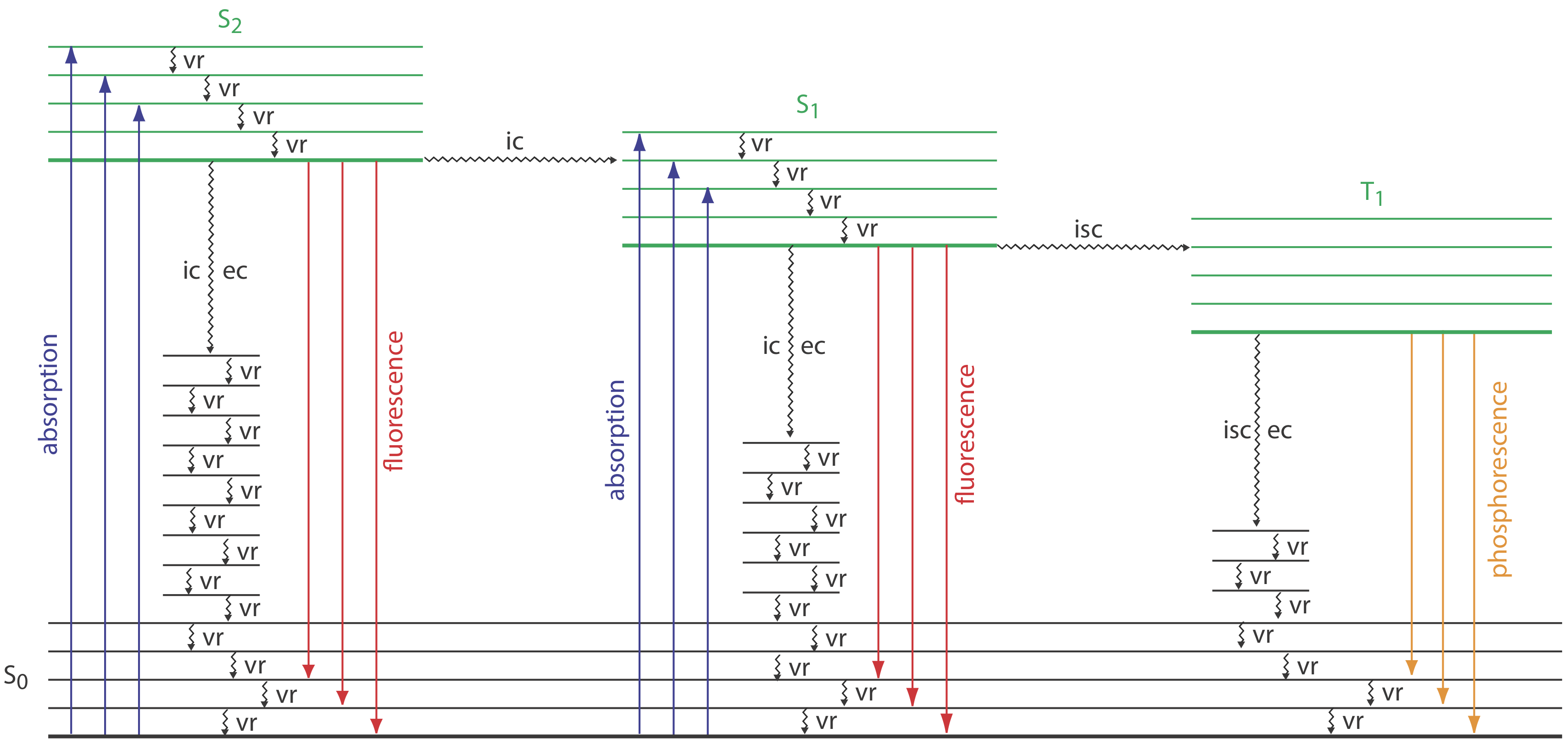
To appreciate the origin of fluorescence and phosphorescence we must consider what happens to a molecule following the absorption of a photon. Let’s assume the molecule initially occupies the lowest vibrational energy level of its electronic ground state, which is the singlet state labeled S0 in Figure \(\PageIndex{2}\). Absorption of a photon excites the molecule to one of several vibrational energy levels in the first excited electronic state, S1, or the second electronic excited state, S2, both of which are singlet states. Relaxation to the ground state occurs by a number of mechanisms, some of which result in the emission of a photon and others that occur without the emission of a photon. These relaxation mechanisms are shown in Figure \(\PageIndex{2}\). The most likely relaxation pathway from any excited state is the one with the shortest lifetime.
Deactivation Processes
A molecule in an excited state can return to its ground state in a variety of ways that we collectively call deactivation processes.
Radiationless Deactivation
When a molecule relaxes without emitting a photon we call the process radiationless deactivation. One example of radiationless deactivation is vibrational relaxation, in which a molecule in an excited vibrational energy level loses energy by moving to a lower vibrational energy level in the same electronic state. Vibrational relaxation is very rapid, with an average lifetime of <10–12 s. Because vibrational relaxation is so efficient, a molecule in one of its excited state’s higher vibrational energy levels quickly returns to the excited state’s lowest vibrational energy level.
Another form of radiationless deactivation is an internal conversion in which a molecule in the ground vibrational level of an excited state passes directly into a higher vibrational energy level of a lower energy electronic state of the same spin state. By a combination of internal conversions and vibrational relaxations, a molecule in an excited electronic state may return to the ground electronic state without emitting a photon. A related form of radiationless deactivation is an external conversion in which excess energy is transferred to the solvent or to another component of the sample’s matrix.
Let’s use Figure \(\PageIndex{2}\) to illustrate how a molecule can relax back to its ground state without emitting a photon. Suppose our molecule is in the highest vibrational energy level of the second electronic excited state. After a series of vibrational relaxations brings the molecule to the lowest vibrational energy level of S2, it undergoes an internal conversion into a higher vibrational energy level of the first excited electronic state. Vibrational relaxations bring the molecule to the lowest vibrational energy level of S1. Following an internal conversion into a higher vibrational energy level of the ground state, the molecule continues to undergo vibrational relaxation until it reaches the lowest vibrational energy level of S0.
A final form of radiationless deactivation is an intersystem crossing in which a molecule in the ground vibrational energy level of an excited electronic state passes into one of the higher vibrational energy levels of a lower energy electronic state with a different spin state. For example, an intersystem crossing is shown in Figure \(\PageIndex{2}\) between the singlet excited state S1 and the triplet excited state T1.
Variables that Affect Fluorescence
Fluorescence occurs when a molecule in an excited state’s lowest vibrational energy level returns to a lower energy electronic state by emitting a photon. Because molecules return to their ground state by the fastest mechanism, fluorescence is observed only if it is a more efficient means of relaxation than a combination of internal conversions and vibrational relaxations.
A quantitative expression of fluorescence efficiency is the fluorescent quantum yield, \(\Phi_f\), which is the fraction of excited state molecules that return to the ground state by fluorescence. The fluorescent quantum yields range from 1 when every molecule in an excited state undergoes fluorescence, to 0 when fluorescence does not occur.
The intensity of fluorescence, If, is proportional to the amount of radiation absorbed by the sample, P0 – PT, and the fluorescence quantum yield
\[I_{f}=k \Phi_{f}\left(P_{0}-P_{\mathrm{T}}\right) \label{10.1} \]
where k is a constant that accounts for the efficiency of collecting and detecting the fluorescent emission. From Beer’s law we know that
\[\frac{P_{\mathrm{T}}}{P_{0}}=10^{-\varepsilon b C} \label{10.2} \]
where C is the concentration of the fluorescing species. Solving Equation \ref{10.2} for PT and substituting into Equation \ref{10.1} gives, after simplifying
\[I_{f}=k \Phi_{f} P_{0}\left(1-10^{-\varepsilon b C}\right) \label{10.3} \]
When \(\varepsilon bC\) < 0.01, which often is the case when the analyte's concentration is small, Equation \ref{10.3} simplifies to
\[I_{f}=2.303 k \Phi_{f} \varepsilon b C P_{0}=k^{\prime} P_{0} \label{10.4} \]
where k′ is a collection of constants. The intensity of fluorescence, therefore, increases with an increase in the quantum efficiency, the source’s incident power, and the molar absorptivity and the concentration of the fluorescing species.
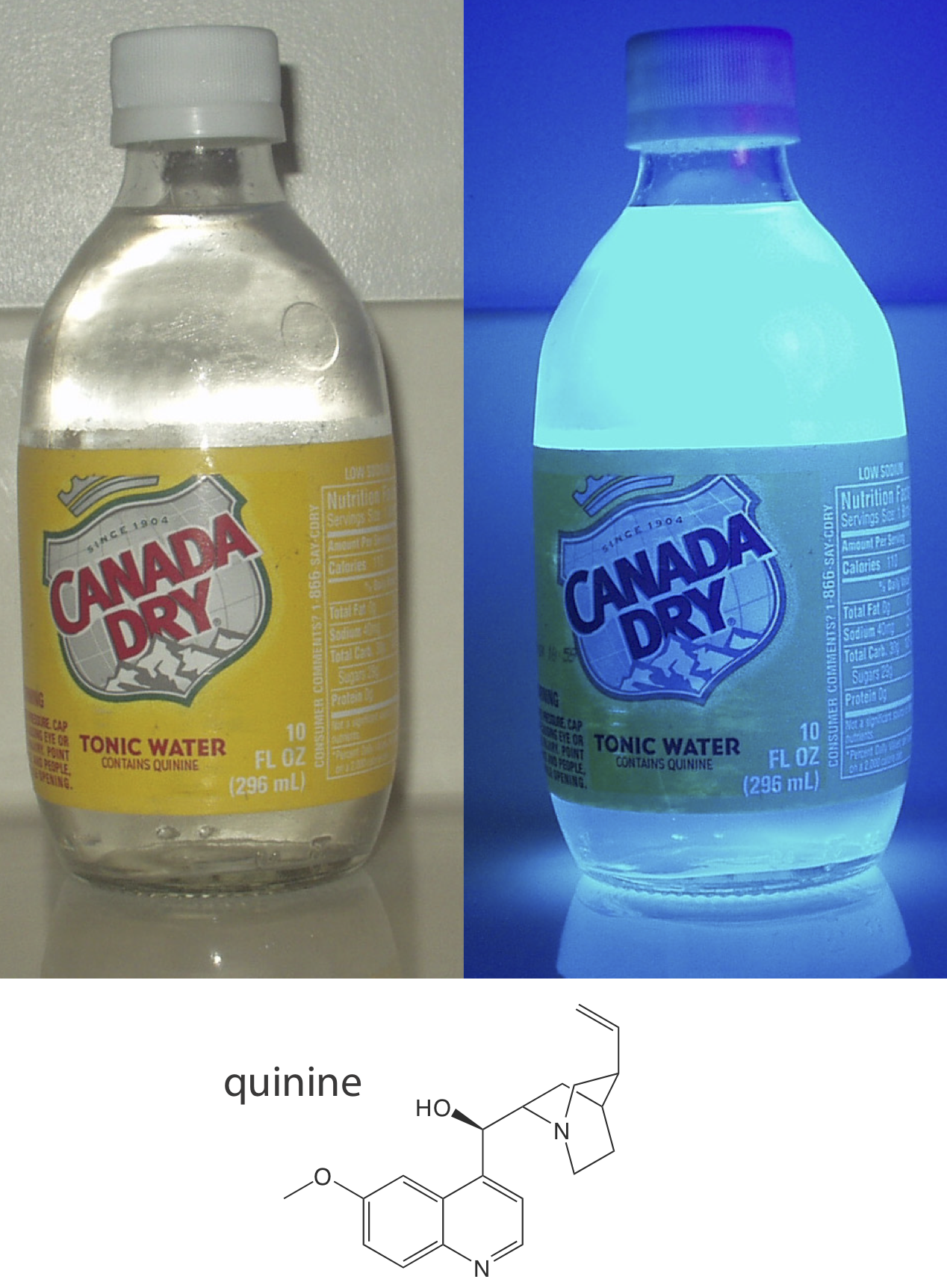
Fluorescence generally is observed when the molecule’s lowest energy absorption is a \(\pi \rightarrow \pi^*\) transition, although some \(n \rightarrow \pi^*\) transitions show weak fluorescence. Many unsubstituted, nonheterocyclic aromatic compounds have a favorable fluorescence quantum yield, although substitutions on the aromatic ring can effect \(\Phi_f\) significantly. For example, the presence of an electron-withdrawing group, such as –NO2, decreases \(\Phi_f\), while adding an electron-donating group, such as –OH, increases \(\Phi_f\). Fluorrescence also increases for aromatic ring systems and for aromatic molecules with rigid planar structures. Figure \(\PageIndex{3}\) shows the fluorescence of quinine under a UV lamp.
A molecule’s fluorescent quantum yield also is influenced by external variables, such as temperature and solvent. Increasing the temperature generally decreases \(\Phi_f\) because more frequent collisions between the molecule and the solvent increases external conversion. A decrease in the solvent’s viscosity decreases \(\Phi_f\) for similar reasons. For an analyte with acidic or basic functional groups, a change in pH may change the analyte’s structure and its fluorescent properties.
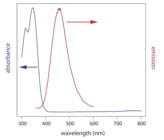
As shown in Figure \(\PageIndex{3}\), fluorescence may return the molecule to any of several vibrational energy levels in the ground electronic state. Fluorescence, therefore, occurs over a range of wavelengths. Because the change in energy for fluorescent emission generally is less than that for absorption, a molecule’s fluorescence spectrum is shifted to higher wavelengths than its absorption spectrum.
Variables that Affect Phosphorescence
A molecule in a triplet electronic excited state’s lowest vibrational energy level normally relaxes to the ground state by an intersystem crossing to a singlet state or by an external conversion. Phosphorescence occurs when the molecule relaxes by emitting a photon. As shown in Figure \(\PageIndex{2}\), phosphorescence occurs over a range of wavelengths, all of which are at lower energies than the molecule’s absorption band. The intensity of phosphorescence, \(I_p\), is given by an equation similar to Equation \ref{10.4} for fluorescence
\[\begin{align} I_{P} &= 2.303 k \Phi_{P} \varepsilon b C P_{0} \nonumber \\[4pt] &= k^{\prime} P_{0} \label{10.5} \end{align}\]
where \(\Phi_p\) is the phosphorescence quantum yield.
Phosphorescence is most favorable for molecules with \(n \rightarrow \pi^*\) transitions, which have a higher probability for an intersystem crossing than \(\pi \rightarrow \pi^*\) transitions. For example, phosphorescence is observed with aromatic molecules that contain carbonyl groups or heteroatoms. Aromatic compounds that contain halide atoms also have a higher efficiency for phosphorescence. In general, an increase in phosphorescence corresponds to a decrease in fluorescence.
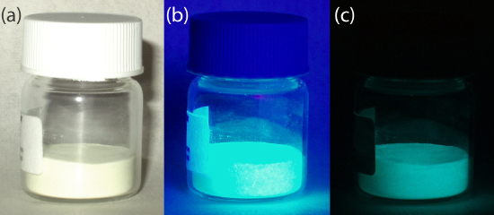
Because the average lifetime for phosphorescence can be quite long, ranging from 10–4–104 s, the phosphorescent quantum yield usually is quite small. An improvement in \(\Phi_p\) is realized by decreasing the efficiency of external conversion. This is accomplished in several ways, including lowering the temperature, using a more viscous solvent, depositing the sample on a solid substrate, or trapping the molecule in solution. Figure \(\PageIndex{4}\) shows an example of phosphorescence.
Emission and Excitation Spectra
Photoluminescence spectra are recorded by measuring the intensity of emitted radiation as a function of either the excitation wavelength or the emission wavelength. An excitation spectrum is obtained by monitoring emission at a fixed wavelength while varying the excitation wavelength. When corrected for variations in the source’s intensity and the detector’s response, a sample’s excitation spectrum is nearly identical to its absorbance spectrum. The excitation spectrum provides a convenient means for selecting the best excitation wavelength for a quantitative or qualitative analysis.
In an emission spectrum a fixed wavelength is used to excite the sample and the intensity of emitted radiation is monitored as function of wavelength. Although a molecule has a single excitation spectrum, it has two emission spectra, one for fluorescence and one for phosphorescence. Figure \(\PageIndex{5}\) shows the UV absorption spectrum and the UV fluorescence emission spectrum for quinine.