7.3: Wavelength Selectors

In Nessler’s original colorimetric method for ammonia, which was described at the beginning of the chapter, the sample and several standard solutions of ammonia are placed in separate tall, flat-bottomed tubes. As shown in Figure \(\PageIndex{1}\), after adding the reagents and allowing the color to develop, the analyst evaluates the color by passing ambient light through the bottom of the tubes and looking down through the solutions. By matching the sample’s color to that of a standard, the analyst is able to determine the concentration of ammonia in the sample.

Figure \(\PageIndex{1}\). Nessler’s original method for comparing the color of two solutions. Natural light passes upwards through the samples and standards and the analyst views the solutions by looking down toward the light source. The top view, shown on the right, is what the analyst sees. To determine the analyte’s concentration, the analyst exchanges standards until the two colors match.

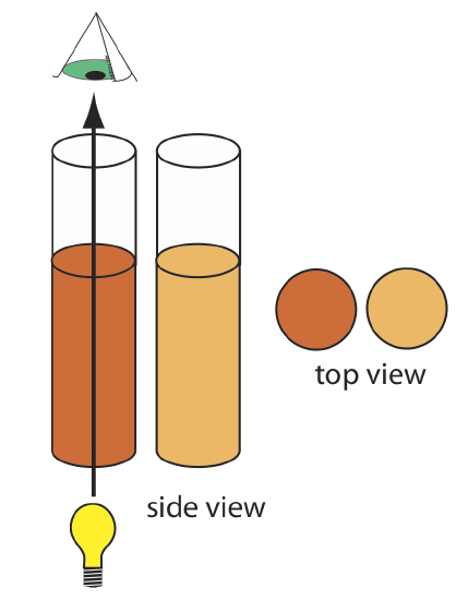
In Figure \(\PageIndex{1}\) every wavelength of light from the source passes through the sample. This is not a problem if there is only one absorbing species in the sample. If the sample contains two components, then a quantitative analysis using Nessler’s original method is impossible unless the standards contains the second component at the same concentration as in the sample.

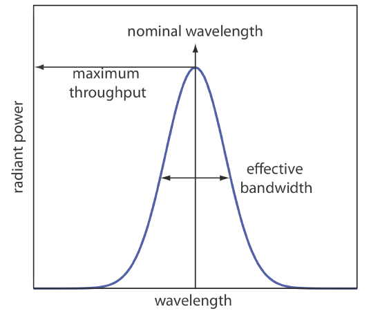
To overcome this problem, we want to select a wavelength that only the analyte absorbs. Unfortunately, we can not isolate a single wavelength of radiation from a continuum source, although we can narrow the range of wavelengths that reach the sample. As seen in Figure \(\PageIndex{2}\), a wavelength selector always passes a narrow band of radiation characterized by a nominal wavelength, an effective bandwidth, and a maximum throughput of radiation. The effective bandwidth is defined as the width of the radiation at half of its maximum throughput.

Figure \(\PageIndex{2}\). Radiation exiting a wavelength selector showing the band’s nominal wavelength and its effective bandwidth.

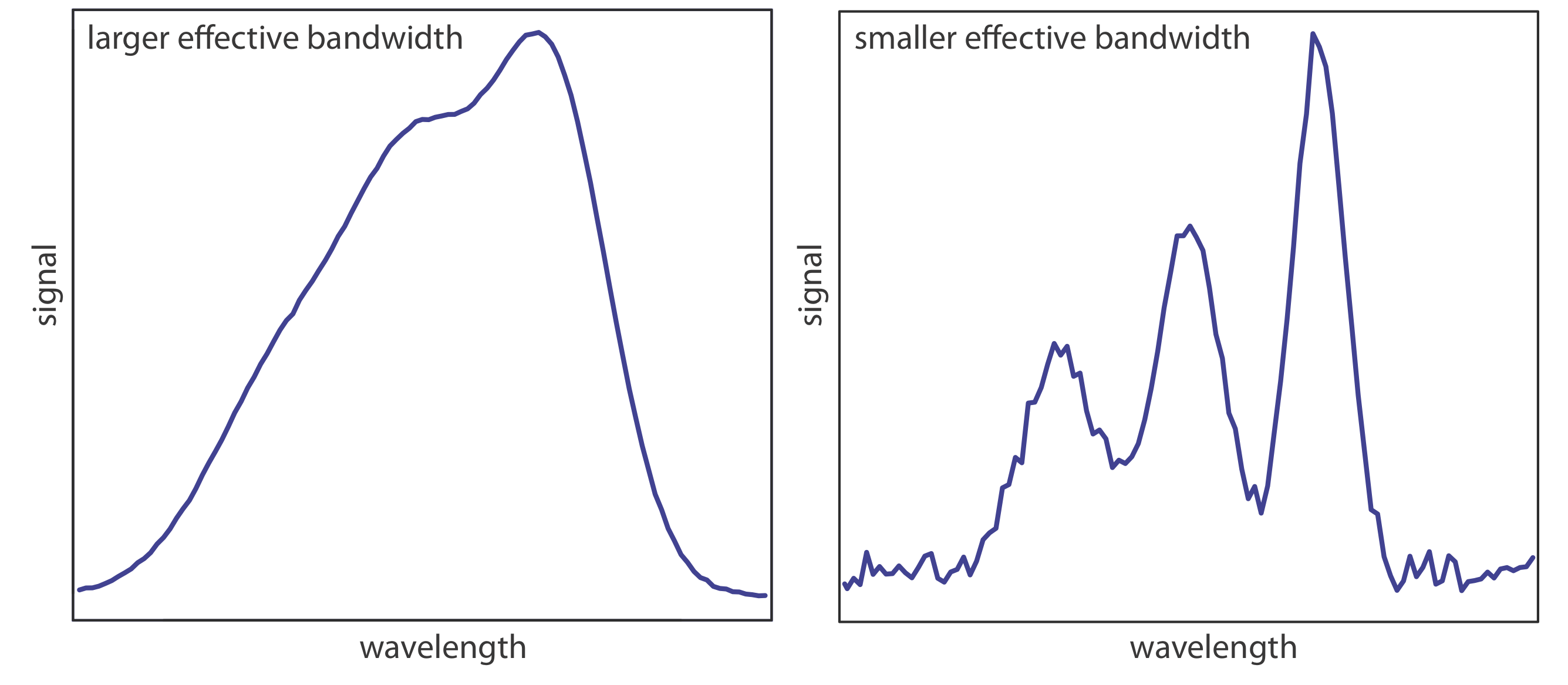
The ideal wavelength selector has a high throughput of radiation and a narrow effective bandwidth. A high throughput is desirable because the more photons that pass through the wavelength selector, the stronger the signal and the smaller the background noise. A narrow effective bandwidth provides a higher resolution, with spectral features separated by more than twice the effective bandwidth being resolved. As shown in Figure \(\PageIndex{3}\), these two features of a wavelength selector often are in opposition. A larger effective bandwidth favors a higher throughput of radiation, but provide less resolution. Decreasing the effective bandwidth improves resolution, but at the cost of a noisier signal [Jiang, S.; Parker, G. A. Am. Lab. 1981, October, 38–43]. For a qualitative analysis, resolution usually is more important than noise and a smaller effective bandwidth is desirable; however, in a quantitative analysis less noise usually is desirable.

Figure \(\PageIndex{3}\). Example showing the effect of the wavelength selector’s effective bandwidth on resolution and noise. The spectrum with the smaller effective bandwidth (on the right) has a better resolution, allowing us to see the presence of three peaks, but at the expense of a noisier signal. The spectrum with the larger effective bandwidth (on the left) has less noise, but at the expense of less resolution between the three peaks.

Filters

The simplest method for isolating a narrow band of radiation is to use an absorption or interference filter.

Absorption Filters

As their name suggests, absorption filters work by selectively absorbing radiation from a narrow region of the electromagnetic spectrum. A simple example of an absorption filter is a piece of colored glass or polymer film. A purple filter, for example, removes the complementary color green from 500–560 nm. Commercially available absorption filters provide effective bandwidths of 30–250 nm, although the throughput at the low end of this range often is only 10% of the source’s emission intensity. Interference filters are more expensive than absorption filters, but have narrower effective bandwidths, typically 10–20 nm, with maximum throughputs of at least 40%. The latter value suggests that an important limitation to an absorption filter is that it may significantly reduce the amount of light from the source that reaches the sample and the detector. Figure \(\PageIndex{4}\) shows an example of a filter holder with filters that pass bands of light centered at 440 nm, 490 nm, or 550 nm.

Figure \(\PageIndex{4}\): The photo on the left shows a filter holder with three filters in place. The photo on the right shows a filter that passes green light centered at 550 nm and a filter that passes blue light centered at 440 nm.

Interference Filters

An interference filter consists of a transparent dielectric material, such as CaF₂, which is sandwiched between two glass plates, each coated with a thin, semitransparent metal film (\(\PageIndex{5}a\)). When a continuous source of light passes through the interference filter it undergoes constructive and destructive interference that isolates and passes a narrow band of light centered at a wavelength that satisfies Equation \ref{lambda}

\[\lambda = \frac{2nb}{m} \label{lambda} \]

where \(n\) is the refractive index of the dielectric material, \(b\) is the thickness of the dielectric material, and \(m\) is the order of the interference (typically first-order). Figure \(\PageIndex{5}b\) shows the result of passing the emission from a green LED—a continuous source that emits light from approximately 500 nm to 650 nm—through an interference filter that produces an effective bandwidth of a few nanometers. In this case, a 210 nm thick film with a refractive index of 1.35 passes light centered at a wavelength of

\[\lambda = \frac{2 \times 1.35 \times 210 \text{ nm}}{1} = 567 \text{ nm} \nonumber \]

Figure \(\PageIndex{5}\). The structure of an Interference filter is shown in (a) and consists of a thin dielectric film sandwiched between two glass plates coated with a thin metal film that allows some of the source's light to pass through the film while reflecting the remainder of the light. Because the light traverses different distances through the dielectric, only light with a wavelength that satisfies Equation \ref{lambda} passes through the filter, resulting in a narrow effective bandwith.

Monochromators

A filter has one significant limitation—because a filter has a fixed nominal wavelength, if we need to make measurements at two wavelengths, then we must use two filters. A monochromator is an alternative method for selecting a narrow band of radiation that also allows us to continuously adjust the band’s nominal wavelength. Monochromators are classified as either fixed-wavelength or scanning. In a fixed-wavelength monochromator we select the wavelength by manually rotating the grating. Normally a fixed-wavelength monochromator is used for a quantitative analysis where measurements are made at one or two wavelengths. A scanning monochromator includes a drive mechanism that continuously rotates the grating, which allows successive wavelengths of light to exit from the monochromator. A scanning monochromator is used to acquire a spectrum, and, when operated in a fixed-wavelength mode, for a quantitative analysis.

The construction of a typical monochromator is shown in Figure \(\PageIndex{6}\). Radiation from the source enters the monochromator through an entrance slit. The radiation is collected by a collimating mirror or lens, which focuses a parallel beam of radiation to a diffraction grating (left) or a prism (right), that disperses the radiation in space. A second mirror or lens focuses the radiation onto a planar surface that contains an exit slit. Radiation exits the monochromator and passes to the detector. As shown in Figure \(\PageIndex{6}\), a monochromator converts a polychromatic source of radiation at the entrance slit to a monochromatic source of finite effective bandwidth at the exit slit. The choice of which wavelength exits the monochromator is determined by rotating the diffraction grating or prism. A narrower exit slit provides a smaller effective bandwidth and better resolution than does a wider exit slit, but at the cost of a smaller throughput of radiation.

Figure \(\PageIndex{6}\). Examples of two types of monochromators: a diffraction grating monochromator an the left and a prism monochromator on the right.

Polychromatic means many colored. Polychromatic radiation contains many different wavelengths of light. Monochromatic means one color, or one wavelength. Although the light exiting a monochromator is not strictly of a single wavelength, its narrow effective bandwidth allows us to think of it as monochromatic.

Monochromators Based on Prisms

Although prism monochromators were once in common use, they have mostly been replaced by diffraction gratings. There are several reasons for this. One reason is that diffraction gratings are much less expensive to manufacture. A second reason is that a diffraction grating provides a linear dispersion of of wavelengths along the focal plane of the exit slit, which means the resolution between adjacent wavelengths is the same throughout the source's optical range. A prism, on the other hand, provides a greater resolution at shorter wavelengths than it does a longer wavelengths.

Monochromators Based on Diffraction Gratings

The inset in the diffraction grating monochromator in Figure \(\PageIndex{6}\) shows the general saw-toothed pattern of a diffraction grating, which consists of a series of grooves with broad surfaces exposed to light from the source. As shown in Figure \(\PageIndex{7}\), parallel beams of source radiation (shown in blue) from the monochromator's collimating mirror strike the surface of the diffraction grating and are reflected back (shown in green) toward the monochromator's focusing mirror and the detector. The parallel beams from the source strike the diffraction grating at an incident angle \(i\) relative to the grating normal, which is a line perpendicular to the diffraction grating's base. The parallel beams bounce back toward the detector do so at a reflected angle \(r\) to the grating normal.

Figure \(\PageIndex{7}\). Illustration of how a monochromator's diffraction grating works to convert a beam of polychromatic light at the monochromator's entrance slit into a monochromatic beam of light at the monochromator's exit slit. Rotating the diffraction grating, changes the angles \(i\) and \(r\) and, therefore, the wavelength of light that exits the monochromator. The diffraction grating illustrated here is known as an echellette-type grating.

Constructive interference between the reflected beams occurs if their path lengths differ by an integer multiple of the incident beam's wavelength (\(n \lambda\)), where \(n\) is the diffraction order. A close examination of Figure \(\PageIndex{7}\) shows that the difference in the distance traveled by two parallel beams of light, identified as 1 and 2, that strike adjacent grooves on the diffraction grating is equal to the sum of the line segments \(\overline{CB}\) and \(\overline{BD}\), both shown in red; thus

\[n \lambda = \overline{CB} + \overline{BD}  \]

The incident angle, \(i\), is equal to the angle CAB and the reflected angle, \(r\), is equal to the angle DAB, which means we can write the following two equations

\[\overline{CB} = d \sin{i} \]

\[\overline{BD} = d \sin{r}  \]

where \(d\) is the distance between the diffraction grating's grooves. Substituting back gives

\[n \lambda = d(\sin{i} + \sin{r}) \label{nlambda} \]

which allows us to calculate the angle at which we can detect a wavelength of interest, \(r\), given the angle of incidence from the source, \(i\), and the number of grooves per mm (or the distance between grooves).

Example \(\PageIndex{1}\)

At what angle can we detect light of 650 nm using a diffraction grating with 1500 gooves per mm if the incident radiation is at an angle of \(50^{\circ}\) to the grating normal? Assume that this is a first-order diffraction.

Solution

The distance between the grooves is

\[d = \frac{1 \text{ mm}}{1500 \text{ grooves}} \times \frac{10^6 \text{ nm}}{\text{mm}} = 666.7 \text{ nm} \nonumber \]

To find the angle, we begin with

\[ n \lambda = 1 \times 650 \text{ nm} = d(\sin{i} + \sin{r}) = 666.7 \text{ nm} \times (\sin{(50)} + \sin{r}) \nonumber \]

\[0.9750 = 0.7660 + \sin{r} \nonumber \]

\[0.2090 = \sin{r} \nonumber \]

\[ r = 12.1^{\circ} \nonumber \]

Performance Characteristics of a Monochromator

The quality of a monochromator depends on several key factors: the purity of the light that emerges from the exit slit, the power of the light that emerges from the exit slit, and the resolution between adjacent wavelengths.

Spectral Purity

The radiation that emerges from a monochromator is pure if it (a) arises from the source and if it (b) follows the optical path from the entrance slit to the exit slit. Stray radiation that enters the monochromator from openings other than the entrance slit—perhaps through small imperfections in the joints—or that reaches the exit slit after scattering from imperfections in the optical components or dust, serves as a contaminant in that the power measured at the detector has a component at the monochromator's analytical wavelength and a component from the stray radiation that includes radiation at other wavelengths.

Power

The amount of radiant energy that exits the monochromator and reaches the detector in a unit time is power. The greater the power, the better the resulting signal-to-noise ratio. The more radiation that enters the monochromator and is gathered by the collimating mirror, the greater the amount of radiation that exits the monochromator and the greater the power at the detector. The ability of a monochromator to collect radiation is defined by its \(f/number\). As shown in Figure \(\PageIndex{8}\), the smaller the \(f/number\), the greater the area and the greater the power. The light-gathering power increases as the inverse square of the \(f/number\); thus, a monochromator rated as \(f/2\) gathers \(4 \times\) as much radiation as a monochromator rated as \(f/4\).

Figure \(\PageIndex{8}\). Relationship between the light-gathering power of a monochromator and its \(f/number\).

Resolution

To separate two wavelengths of light and detect them separately, it is necessary to to disperse them over a sufficient distance. The angular dispersion of a monochromator is defined as the change in the angle of reflection (see the angle \(r\) in Figure \(\PageIndex{7}\)) for a change in wavelength, or \(dr/d\lambda\). Taking the derivative of Equation \ref{nlambda} for a fixed angle of incidence (see the angle \(i\) in Figure \(\PageIndex{7}\)) gives the angular dispersion as

\[ \frac{dr}{d \lambda} = \frac{n}{d \cos{r}} \label{angdisp} \]

where \(n\) is the diffraction order. The linear dispersion of radiation, \(D\), gives the change in wavelength as a function of \(y\), the distance along the focal plane of the monochromator's exit slit; this is related to the angular dispersion by

\[D = \frac{dy}{d \lambda} = \frac{F dr}{d \lambda} \label{lineardisp} \]

where \(F\) is the focal length. Because we are interested in wavelength, it is convenient to take the inverse of Equation \ref{lineardisp}

\[D^{-1} = \frac{d \lambda}{dy} = \frac{1}{F} \times \frac{d \lambda}{dr} \label{invlineardisp} \]

where \(D^{-1}\) is the reciprocal linear dispersion. Substituting Equation \ref{angdisp} into Equation \ref{invlineardisp} gives

\[D^{-1} = \frac{d \lambda}{dy} = \frac{d \cos{r}}{nF}  \]

which simplifies to

\[D^{-1} = \frac{d}{nF}  \]

for angles \(r < 20^{\circ}\) where \(\cos{r} \approx 1\). Because the linear dispersion of radiation along the monochromator's exit slit is independent of wavelength, the ability to resolve two wavelengths is the same across the spectrum of wavelengths.

Another way to report a monochromator's ability to distinguish between two closely spaced wavelengths is its resolving power, \(R\), which is defined as

\[R = \frac{\lambda}{\Delta \lambda} = n N \nonumber \]

where \(\lambda\) is the average of the two wavelengths, \(\Delta \lambda\) is the difference in their values and \(N\) is the number of grooves on the diffraction grating that are exposed to the radiation from the collimating mirror. The greater the number of grooves, the greater the resolving power.

Monochromator Slits

A monochromator has two sets of slits: an entrance slit that brings radiation from the source into the monochromator and an exit slit that passes the radiation from the monochromator to the detector. Each slit consists of two metal plates with sharp, beveled edges separated by a narrow gap that forms a rectangular window and which is aligned with the focal plane of the collimating mirror. Figure \(\PageIndex{9}\) shows a set of four slits from a monochromator taken from an atomic absorption spectrophotometer. From bottom-to-top, the slits have widths, \(w\), of 2.0 mm, 1.0 mm, 0.5 mm, and 0.2 mm.

Figure \(\PageIndex{9}\). Photo showing a set of four entrance slits to a monochromator from an atomic absorption spectrometer. From bottom-to-top they have widths of 2.0 mm, 1.0 mm, 0.5 mm, and 0.2 mm. The monochromator's exit slits are identical and. For this monochromator, the operator selects the slit width for the entrance slits and the exit is automatically set to the same width.

Effect of Slits on Monochromatic Radiation

Suppose we have a source of monochromatic radiation with a wavelength of 400.0 nm and that we pass this beam of radiation through a monochromator that has entrance and exit slits with a width, \(w\), of 1.0 mm and a reciprocal linear dispersion of 1.2 nm/mm. The product of these two variables is called the monochromator's effective bandwidth, \(\Delta \lambda_\text{eff}\), and is given as

\[\Delta \lambda_\text{eff} = w D^{-1} = 1.0 \text{ mm} \times 1.2 \text{ nm/mm} = 1.2 \text{ nm} \]

The width of the beam in units of wavelength, therefore, is 1.2 nm. In this case, as shown in Figure \(\PageIndex{10}\), if we scan the monochromator, our beam of monochromatic radiation will first enter the exit slit at a wavelength setting of 398.8 nm and will fully exit the slit at a wavelength setting of 401.2 nm. In between these limits a portion of the beam is blocked and only a portion of the beam passes through the exit slit and reaches the detector. For example, when the monochromator is set to 399.4 nm or 400.6 nm, half of ther beam reaches the detector with a power of \(0.5\times P\). If we monitor the power at the detector as a function of wavelength, we obtain the profile shown at the bottom of Figure \(\PageIndex{10}\). The monochromator's bandwidth encompasses the range of wavelengths over which some portion of the beam of radiation passes through the exit slit.

Figure \(\PageIndex{10}\): Illustration showing the relationship between effective bandwidth of a monochromatic source of radiation and the width of a monochromator's exit slit.

Effect of Slit Width on Resolution

Suppose we have a source of radiation that consists of precisely three wavelengths—399.4 nm, 400.0 nm, and 400.6 nm—and we pass them through a monochromator with an effective bandwidth of 1.2 nm. Using the analysis from the previous section, the radiation with a wavelength of 399.4 nm passes through the monochromator's exit slit for any wavelength setting between 398.8 and 400.0 nm, which means it overlaps with the radiation with a wavelength of 400.0 nm. The same is true for the radiation with a wavelength of 400.6 nm, which also overlaps with the radiation with a wavelength of 400.0 nm. As shown in Figure \(\PageIndex{11}a\), we cannot resolve the three monochromatic sources of radiation, which appear as a single broad band of radiation. Decreasing the effective bandwidth to one-half of the difference in the wavelengths of the adjacent sources of radiation produces, as shown in Figure \(\PageIndex{11}b\), baseline resolution of the individual sources of wavelength. To resolve the sources of radiation with wavelengths of 399.4 nm and 400.0 nm using a monochromator with a reciprical linear dispersion of 1.2 nm/mm requires an effective bandwidth of

\[\Delta \lambda_\text{eff} = 0.5 \times (400.0 \text{ nm} - 399.4 \text{ nm}) = 0.3 \text{ nm} \nonumber \]

and a slit width of

\[w = \frac{\Delta \lambda_\text{eff}}{D^{-1}} = \frac{0.3 \text{ nm}}{1.2 \text{nm/mm}} = 0.25 \text{ mm} \nonumber \]

Figure \(\PageIndex{11}\): Illustration showing (a) the inability of a monochromator with an effective bandwidth of 1.2 nm to resolve three lines with wavelengths of 399.4 nm, 400.0 nm, and 400.6 nm. Decreasing the effective bandwidth to 0.3 nm, as in (b), allows for complete resolution of the three lines.

Choosing a Slit Width

The choice of slit width always involves a trade-off between increasing the radiant power that reaches the detector by using a wide slit width, which improves the signal-to-noise ratio, and improving the resolution between closely spaced peaks, which requires a narrow slit width. Figure \(\PageIndex{3}\) illustrates this trade-off. Ultimately, the needs of the analyst will dictate the choice of slit width.