
7.2: Sources of Radiation
- Page ID
- 366607

\( \newcommand{\vecs}[1]{\overset { \scriptstyle \rightharpoonup} {\mathbf{#1}} } \)
\( \newcommand{\vecd}[1]{\overset{-\!-\!\rightharpoonup}{\vphantom{a}\smash {#1}}} \)
\( \newcommand{\id}{\mathrm{id}}\) \( \newcommand{\Span}{\mathrm{span}}\)
( \newcommand{\kernel}{\mathrm{null}\,}\) \( \newcommand{\range}{\mathrm{range}\,}\)
\( \newcommand{\RealPart}{\mathrm{Re}}\) \( \newcommand{\ImaginaryPart}{\mathrm{Im}}\)
\( \newcommand{\Argument}{\mathrm{Arg}}\) \( \newcommand{\norm}[1]{\| #1 \|}\)
\( \newcommand{\inner}[2]{\langle #1, #2 \rangle}\)
\( \newcommand{\Span}{\mathrm{span}}\)
\( \newcommand{\id}{\mathrm{id}}\)
\( \newcommand{\Span}{\mathrm{span}}\)
\( \newcommand{\kernel}{\mathrm{null}\,}\)
\( \newcommand{\range}{\mathrm{range}\,}\)
\( \newcommand{\RealPart}{\mathrm{Re}}\)
\( \newcommand{\ImaginaryPart}{\mathrm{Im}}\)
\( \newcommand{\Argument}{\mathrm{Arg}}\)
\( \newcommand{\norm}[1]{\| #1 \|}\)
\( \newcommand{\inner}[2]{\langle #1, #2 \rangle}\)
\( \newcommand{\Span}{\mathrm{span}}\) \( \newcommand{\AA}{\unicode[.8,0]{x212B}}\)
\( \newcommand{\vectorA}[1]{\vec{#1}} % arrow\)
\( \newcommand{\vectorAt}[1]{\vec{\text{#1}}} % arrow\)
\( \newcommand{\vectorB}[1]{\overset { \scriptstyle \rightharpoonup} {\mathbf{#1}} } \)
\( \newcommand{\vectorC}[1]{\textbf{#1}} \)
\( \newcommand{\vectorD}[1]{\overrightarrow{#1}} \)
\( \newcommand{\vectorDt}[1]{\overrightarrow{\text{#1}}} \)
\( \newcommand{\vectE}[1]{\overset{-\!-\!\rightharpoonup}{\vphantom{a}\smash{\mathbf {#1}}}} \)
\( \newcommand{\vecs}[1]{\overset { \scriptstyle \rightharpoonup} {\mathbf{#1}} } \)
\( \newcommand{\vecd}[1]{\overset{-\!-\!\rightharpoonup}{\vphantom{a}\smash {#1}}} \)
\(\newcommand{\avec}{\mathbf a}\) \(\newcommand{\bvec}{\mathbf b}\) \(\newcommand{\cvec}{\mathbf c}\) \(\newcommand{\dvec}{\mathbf d}\) \(\newcommand{\dtil}{\widetilde{\mathbf d}}\) \(\newcommand{\evec}{\mathbf e}\) \(\newcommand{\fvec}{\mathbf f}\) \(\newcommand{\nvec}{\mathbf n}\) \(\newcommand{\pvec}{\mathbf p}\) \(\newcommand{\qvec}{\mathbf q}\) \(\newcommand{\svec}{\mathbf s}\) \(\newcommand{\tvec}{\mathbf t}\) \(\newcommand{\uvec}{\mathbf u}\) \(\newcommand{\vvec}{\mathbf v}\) \(\newcommand{\wvec}{\mathbf w}\) \(\newcommand{\xvec}{\mathbf x}\) \(\newcommand{\yvec}{\mathbf y}\) \(\newcommand{\zvec}{\mathbf z}\) \(\newcommand{\rvec}{\mathbf r}\) \(\newcommand{\mvec}{\mathbf m}\) \(\newcommand{\zerovec}{\mathbf 0}\) \(\newcommand{\onevec}{\mathbf 1}\) \(\newcommand{\real}{\mathbb R}\) \(\newcommand{\twovec}[2]{\left[\begin{array}{r}#1 \\ #2 \end{array}\right]}\) \(\newcommand{\ctwovec}[2]{\left[\begin{array}{c}#1 \\ #2 \end{array}\right]}\) \(\newcommand{\threevec}[3]{\left[\begin{array}{r}#1 \\ #2 \\ #3 \end{array}\right]}\) \(\newcommand{\cthreevec}[3]{\left[\begin{array}{c}#1 \\ #2 \\ #3 \end{array}\right]}\) \(\newcommand{\fourvec}[4]{\left[\begin{array}{r}#1 \\ #2 \\ #3 \\ #4 \end{array}\right]}\) \(\newcommand{\cfourvec}[4]{\left[\begin{array}{c}#1 \\ #2 \\ #3 \\ #4 \end{array}\right]}\) \(\newcommand{\fivevec}[5]{\left[\begin{array}{r}#1 \\ #2 \\ #3 \\ #4 \\ #5 \\ \end{array}\right]}\) \(\newcommand{\cfivevec}[5]{\left[\begin{array}{c}#1 \\ #2 \\ #3 \\ #4 \\ #5 \\ \end{array}\right]}\) \(\newcommand{\mattwo}[4]{\left[\begin{array}{rr}#1 \amp #2 \\ #3 \amp #4 \\ \end{array}\right]}\) \(\newcommand{\laspan}[1]{\text{Span}\{#1\}}\) \(\newcommand{\bcal}{\cal B}\) \(\newcommand{\ccal}{\cal C}\) \(\newcommand{\scal}{\cal S}\) \(\newcommand{\wcal}{\cal W}\) \(\newcommand{\ecal}{\cal E}\) \(\newcommand{\coords}[2]{\left\{#1\right\}_{#2}}\) \(\newcommand{\gray}[1]{\color{gray}{#1}}\) \(\newcommand{\lgray}[1]{\color{lightgray}{#1}}\) \(\newcommand{\rank}{\operatorname{rank}}\) \(\newcommand{\row}{\text{Row}}\) \(\newcommand{\col}{\text{Col}}\) \(\renewcommand{\row}{\text{Row}}\) \(\newcommand{\nul}{\text{Nul}}\) \(\newcommand{\var}{\text{Var}}\) \(\newcommand{\corr}{\text{corr}}\) \(\newcommand{\len}[1]{\left|#1\right|}\) \(\newcommand{\bbar}{\overline{\bvec}}\) \(\newcommand{\bhat}{\widehat{\bvec}}\) \(\newcommand{\bperp}{\bvec^\perp}\) \(\newcommand{\xhat}{\widehat{\xvec}}\) \(\newcommand{\vhat}{\widehat{\vvec}}\) \(\newcommand{\uhat}{\widehat{\uvec}}\) \(\newcommand{\what}{\widehat{\wvec}}\) \(\newcommand{\Sighat}{\widehat{\Sigma}}\) \(\newcommand{\lt}{<}\) \(\newcommand{\gt}{>}\) \(\newcommand{\amp}{&}\) \(\definecolor{fillinmathshade}{gray}{0.9}\)All forms of spectroscopy require a source of energy to place the analyte in an excited state. In absorption and scattering spectroscopy this energy is supplied by photons. Emission and photoluminescence spectroscopy use thermal energy, radiant (photon) energy, or chemical energy to promote the analyte to a suitable excited state. In this section we consider the sources of radiant energy.
Sources of Electromagnetic Radiation
A source of electromagnetic radiation must provide an output that is both intense and stable in the region of interest. Sources of electromagnetic radiation are classified as either continuum or line sources. Table \(\PageIndex{1}\) provides a list of some common sources of electromagnetic radiation.
| source | wavelength region | useful for... |
|---|---|---|
| H2 and D2 lamp | continuum source from 160–380 nm | molecular absorption |
| tungsten lamp | continuum source from 320–2400 nm | molecular absorption |
| Xe arc lamp | continuum source from 200–1000 nm | molecular fluorescence |
| nernst glower | continuum source from 0.4–20 µm | molecular absorption |
| globar | continuum source from 1–40 µm | molecular absorption |
| nichrome wire | continuum source from 0.75–20 µm | molecular absorption |
| hollow cathode lamp | line source in UV/Vis | atomic absorption |
| Hg vapor lamp | line source in UV/Vis | molecular fluorescence |
| laser | line source in UV/Vis/IR | atomic and molecular absorption, fluorescence, and scattering |
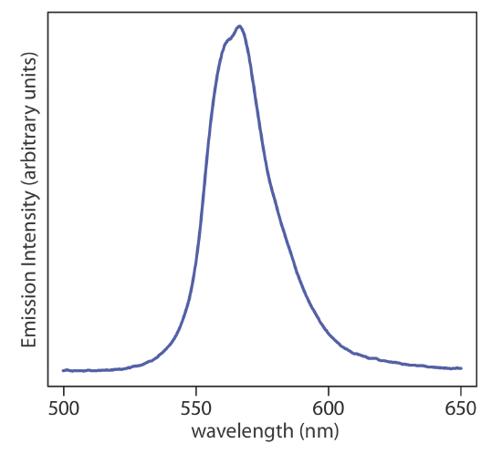
Continuum sources emits radiation over a broad range of wavelengths, with a relatively smooth variation in intensity (Figure \(\PageIndex{1}\)), and are used for molecular absorbance using UV/Vis and IR radiation. Further details on these sources are in Chapters 13 and 16, respectively.
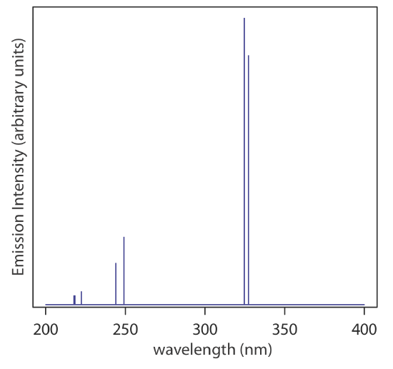
A line source, on the other hand, emits radiation at discrete wavelengths, with broad regions showing no emission lines (Figure \(\PageIndex{2}\)), and are used for atomic absorption, atomic and molecular fluorescence, and Raman spectroscopy. Further details on hollow cathode lamps are included in Chapter 9.
Laser Sources
An important line source of radiation is a laser, which is an acronym for light amplification by stimulated emission of radiation. Laser emission is monochromatic with a narrow bandwidth of just a few micrometers. As suggested by the term amplification, a laser provides a source of high intensity emission. The source of this intensity is embedded in the term stimulated emission, to which we now turn our attention.
How a Laser Works
To understand how a laser works, we need to consider four key ideas: pumping, population inversion, stimulated emission, and light amplification.
Pumping
Emission cannot occur unless we first populate higher energy levels with electrons, which we can accomplish by, for example, the absorption of photons, as shown in Figure \(\PageIndex{3}\). Emission occurs when an electron in a higher energy state relaxes back to a lower energy state by emitting a photon with an energy equal to the difference in the energy between these two states. The process of populating the excited states with electrons is called pumping and is accomplished by using an electrical discharge, by passing an electrical current through the lasing medium, or by absorption of high energy photons. The goal of pumping is to create a large population of excited states.

Population Inversion
Normally the majority of the species we are studying are in their ground electronic state with only a small number of species in an excited electronic state. For a laser to achieve a high intensity of emission, it is necessary to create a situation in which there are more species in the excited state than in the ground state, as shown in Figure \(\PageIndex{4}\) where the non-inverted population has four species in the ground state and two species in the excited state, and where the inverted population has four species in the excited state and two species in the ground state.

Stimulated Emission and Light Amplification
Figure \(\PageIndex{3}\) shows emission of a photon following absorption of a photon of equal energy. No more than one photon is emitted for each photon that is absorbed, with some species in an excited state relaxing to the ground state through non-radiative pathways. This spontaneous emission is a random process, which means that the timing of emission and the direction in which emission occurs are random.
Emission in a laser, as depicted in Figure \(\PageIndex{5}\), is stimulated by a photon with an energy equal to that of the difference in energy between the excited state and the ground state. The interaction of the incoming photon with the excited state results in the excited state's immediate relaxation to the ground state by the emission of a photon. The original photon and the emitted photon are coherent, with identical energies, identical directions, and identical phases. Because two coherent photons are emitted, the amplitude of the emitted radiation is doubled, as we see in Figure \(\PageIndex{5}\); this is what we mean by light amplification.

Laser Systems
As the previous sections suggest, creating a population inversion is the limiting factor in generating radiation from a laser. The two-level system in Figure \(\PageIndex{5}\), which involves a single excited state and a single ground state, cannot create a population inversion because when the ground state and excited state are equal in population, the rate at which excited states are produced through pumping equals the rate at which excited states are lost through emission. To achieve stimulated emission, laser systems use three-level or four-level systems, as outlined in Figure \(\PageIndex{6}\).

In a three-level system, pumping is used to populate the excited states in level two. From level two, an efficient pathway for non-radiative relaxation populates the excited state in level three, which is sufficiently stable to allow for a population inversion. In a four-level system, the population inversion is achieved between level three and level four.
Types of Lasers
Lasers are categorized by the nature of the lasing medium: solid-state crystals, gases, dyes, and semiconductors. Solid-state lasers use a crystalline material, such as aluminum oxide, that contains trace amounts of an element, such as chromium or neodymium, which serves as the actual lasing medium. Gas lasers use gas phase atoms, ions, or molecules as a lasing medium. The lasing medium in a dye laser is a solution of an organic dye molecule. A dye laser typically is capable of emitting light over a broad range of wavelengths, but is tunable to a specific wavelength within that range. Finally, a semiconductor laser uses modified light-emitting diodes as a lasing medium.
| category | lasing medium | wavelengths |
|---|---|---|
| solid state | ruby (0.05% Cr(III) in Al2O3) | 694.3 nm |
| Nd:YAG (neodymium ion in yttrium aluminum garnet | 1054 nm; 532 nm | |
| gas | He/Ne | 632.8 nm |
| Ar+ | 514.5 nm, 488 nm | |
| N2 | 337.1 nm | |
| CO2 | 10.6 µm | |
| dye | rhodamine | 540–680 nm |
| fluorescein | 530–560 nm | |
| cumarin | 490–620 nm | |
| semiconductor | indium gallium nitride | 405 nm |
| aluminum gallium indium phosphide | 635 nm |