3.3: Amplification and Measurement of Signals

In Chapter 1.3 we identified the basic components of an instrument as a probe that interacts with the sample, an input transducer that converts the sample's chemical and/or physical properties into an electrical signal, a signal processor that converts the electrical signal into a form that an output transducer can convert into a numerical or a visual output that we can understand. We can represent this as a sequence of actions that take place within the instrument

\[\text{probe} \rightarrow \text{sample} \rightarrow \text{input transducer} \rightarrow \text{raw data} \rightarrow\text{signal processor} \rightarrow \text{output transducer} \nonumber \]

creating the following general flow of information

\[\text{chemical and/or physical information} \rightarrow \text{electrical information} \rightarrow \text{numerical or visual response} \nonumber \]

As suggested above, information is encoded in two broad ways: as electrical information (such as currents and potentials) and as information in other, non-electrical forms (such as chemical and physical properties). In this section we will consider how we can measure electrical signals.

Current Measurements

In Chapter 7 we will introduce the phototube, seen here in Figure \(\PageIndex{1}\), as a transducer for converting photons of light into an electrical current that we can measure. A photon of light strikes a photoemissive cathode and ejects an electron that is then drawn to an anode that is held a positive potential. The resulting current is our analytical signal. As each photon generates a single electron, the resulting current is small and needs amplifying if it is to be useful to us. Operational amplifiers provide a way to accomplish this amplification.

Figure \(\PageIndex{1}\). Schematic illustration of a phototube. See Chapter 7 for additional details.

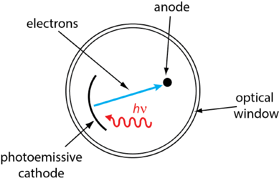
Figure \(\PageIndex{2}\) shows a simple electrical circuit that we can use to amplify and measure a small current. If you compare this to the inverting amplifier circuit in Chapter 3.2, you will see that we are replacing the input voltage and input resistor with the input current, \(I_x\), that we wish to measure.

Figure \(\PageIndex{2}\). Operational amplifier circuit for converting a current into a voltage.

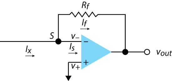
From Kirchoff's current law, we know that at the summing point, \(S\), the current from the transducer is equal to the sum of the current through the feedback loop, \(I_f\), and the current to the op amp's inverting input, \(I_s\).

\[I_x = I_s + I_f \label{iv1} \]

As we learned in the last section, \(I_s \approx 0\), which means \(I_x \approx I_f\). From Ohm's law, we have

\[V_{out} = - I_f \times R_f = -I_x \times R_f \label{iv2} \]

Rearranging to solve for \(I_x\)

\[I_x = - \frac{V_{out}}{R_f} = k V_{out} \label{iv3} \]

shows us that there is a linear relationship between the voltage we measure from the circuit's output and the current that enters the circuit. By choosing to make \(R_f\) large, a small current is converted into a voltage that is easy to measure. In addition, we know from Chapter 2 that the error in measuring the current from the transducer, \(E_x\), is

\[E_x = - \frac{R_m}{R_m + R_l} \times 100 \label{iv4} \]

where \(R_m\) is the resistance of the measuring circuit and \(R_l\) is the resistance of the source, which generally is large. The resistance of the measuring circuit is

\[R_{m} = \frac{R_r}{A_{op}} \label{iv5} \]

If we choose \(R_f\) such that it is similar in magnitude to the op amp's gain, \(A_{op}\), then \(R_m\) is small and the relative error is small as well.

Potential Measurements

From Chapter 2 we know that the error in measuring voltage, \(E_x\), is a function of the resistance of the measuring circuit, \(R_m\), and the resistance of the source, \(R_x\).

\[E_x = \frac{V_m - V_x}{V_x} \times 100 = - \frac{R_m}{R_m + R_x} \times 100 \label{volt1} \]

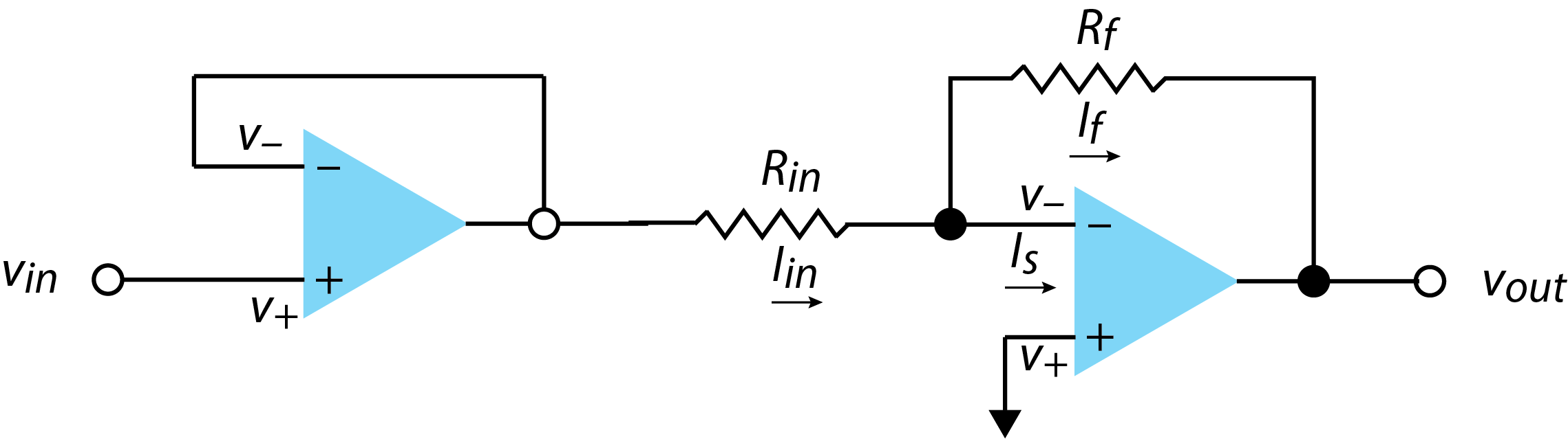
To maintain a small measurement error requires that \(R_x << R_m\). This creates a complication when the voltage source has a high internal resistance, as is the case, for example, when we measure pH using a glass electrode where the internal resistance is on the order of \(10^7 - 10^8 \Omega\) (see Chapter 23 for details about glass electrodes). The inverting amplifier circuit discussed in Chapter 3.2 has a resistance of perhaps \(10^5 \Omega\). To increase \(R_m\), the voltage we wish to measure, \(V_x\), is first run through a voltage follower circuit, where the internal resistance is on the order of \(10^{12} \Omega\), and the output is then run through the inverting amplifier, as seen in Figure \(\PageIndex{3}\). The result is an amplified output voltage measured under conditions where the relative error is small.

Figure \(\PageIndex{3}\). Circuit for measuring voltage that combines a voltage follower and an inverting amplifier.

Comparison of Transducer Outputs

In Chapter 13 we will cover molecular absorption spectroscopy in which we measure the absorbance of sample relative to the absorbance of a reference. A difference amplifier, such as that shown in Figure \(\PageIndex{4}\), allows us to amplify and measure the difference between two voltages. In this circuit, the two voltages, \(v_1\) and \(v_2\), are fed into the op amp's two inputs, \(v_{-}\) and \(v_{+}\), passing through identical resistors. A feedback loop with a resistor connects \(v_1\) to \(v_{out}\) and a resistor identical to that in the feedback loop connects \(v_2\) to the circuit common.

Figure \(\PageIndex{4}\). Circuit used to amplify and measure the difference between two voltages.

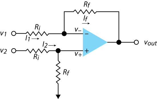
We can use Ohm's law to define the currents \(I_1\) and \(I_f\) as

\[I_1 = \frac{v_1 - v_{-}}{R_i} \label{comp1} \]

\[I_f = \frac{v_{-} - v_{out}}{R_f} \label{comp2} \]

By now you should see that the currents \(I_1\) and \(I_f\) are approximately the same because the op amp's high internal impedence prevents current from flowing into the op amp. Combining Equation \ref{comp1} and Equation \ref{comp2} gives

\[\frac{v_1 - v_{-}}{R_i} = \frac{v_{-} - v_{out}}{R_f} \label{comp3} \]

which we can solve for the voltage at the op amp's inverting input

\[R_f v_1 - R_f v_{-} = R_i v_{-} - R_i V_{out} \label{comp4} \]

\[R_i v_{-} + R_f v_{-} = R_f v_1 + R_i v_{out} \label{comp5} \]

\[v_{-} = \frac{R_f v_1 + R_i v_{out}}{R_i + R_f} \label{comp6} \]

The input to the op amp's noniverting lead is the output of a voltage divider (see Chapter 2) acting on \(v_2\)

\[v_{+} = v_2 \times \left( \frac{R_f}{R_i + R_f} \right) \label{comp7} \]

The feedback loop works to ensure that the inputs to \(v_{-}\) and to \(v_{+}\) are identical; thus

\[\frac{R_f v_1 + R_i v_{out}}{R_i + R_f} = v_2 \times \left( \frac{R_f}{R_i + R_f} \right) \label{comp8} \]

which we can simply to

\[V_1 R_f + V_{out} R_i = V_2 R_f \label{comp9} \]

\[V_{out} = \frac{R_f}{R_i} \times (V_2 - V_1) \label{comp10} \]

The output voltage from the circuit is equal to the difference between the two input voltages, but amplified by the ratio of the resistance of \(R_f\) to \(R_i\).