
3.2: Operational Amplifier Circuits
- Page ID
- 406439

\( \newcommand{\vecs}[1]{\overset { \scriptstyle \rightharpoonup} {\mathbf{#1}} } \)
\( \newcommand{\vecd}[1]{\overset{-\!-\!\rightharpoonup}{\vphantom{a}\smash {#1}}} \)
\( \newcommand{\id}{\mathrm{id}}\) \( \newcommand{\Span}{\mathrm{span}}\)
( \newcommand{\kernel}{\mathrm{null}\,}\) \( \newcommand{\range}{\mathrm{range}\,}\)
\( \newcommand{\RealPart}{\mathrm{Re}}\) \( \newcommand{\ImaginaryPart}{\mathrm{Im}}\)
\( \newcommand{\Argument}{\mathrm{Arg}}\) \( \newcommand{\norm}[1]{\| #1 \|}\)
\( \newcommand{\inner}[2]{\langle #1, #2 \rangle}\)
\( \newcommand{\Span}{\mathrm{span}}\)
\( \newcommand{\id}{\mathrm{id}}\)
\( \newcommand{\Span}{\mathrm{span}}\)
\( \newcommand{\kernel}{\mathrm{null}\,}\)
\( \newcommand{\range}{\mathrm{range}\,}\)
\( \newcommand{\RealPart}{\mathrm{Re}}\)
\( \newcommand{\ImaginaryPart}{\mathrm{Im}}\)
\( \newcommand{\Argument}{\mathrm{Arg}}\)
\( \newcommand{\norm}[1]{\| #1 \|}\)
\( \newcommand{\inner}[2]{\langle #1, #2 \rangle}\)
\( \newcommand{\Span}{\mathrm{span}}\) \( \newcommand{\AA}{\unicode[.8,0]{x212B}}\)
\( \newcommand{\vectorA}[1]{\vec{#1}} % arrow\)
\( \newcommand{\vectorAt}[1]{\vec{\text{#1}}} % arrow\)
\( \newcommand{\vectorB}[1]{\overset { \scriptstyle \rightharpoonup} {\mathbf{#1}} } \)
\( \newcommand{\vectorC}[1]{\textbf{#1}} \)
\( \newcommand{\vectorD}[1]{\overrightarrow{#1}} \)
\( \newcommand{\vectorDt}[1]{\overrightarrow{\text{#1}}} \)
\( \newcommand{\vectE}[1]{\overset{-\!-\!\rightharpoonup}{\vphantom{a}\smash{\mathbf {#1}}}} \)
\( \newcommand{\vecs}[1]{\overset { \scriptstyle \rightharpoonup} {\mathbf{#1}} } \)
\( \newcommand{\vecd}[1]{\overset{-\!-\!\rightharpoonup}{\vphantom{a}\smash {#1}}} \)
\(\newcommand{\avec}{\mathbf a}\) \(\newcommand{\bvec}{\mathbf b}\) \(\newcommand{\cvec}{\mathbf c}\) \(\newcommand{\dvec}{\mathbf d}\) \(\newcommand{\dtil}{\widetilde{\mathbf d}}\) \(\newcommand{\evec}{\mathbf e}\) \(\newcommand{\fvec}{\mathbf f}\) \(\newcommand{\nvec}{\mathbf n}\) \(\newcommand{\pvec}{\mathbf p}\) \(\newcommand{\qvec}{\mathbf q}\) \(\newcommand{\svec}{\mathbf s}\) \(\newcommand{\tvec}{\mathbf t}\) \(\newcommand{\uvec}{\mathbf u}\) \(\newcommand{\vvec}{\mathbf v}\) \(\newcommand{\wvec}{\mathbf w}\) \(\newcommand{\xvec}{\mathbf x}\) \(\newcommand{\yvec}{\mathbf y}\) \(\newcommand{\zvec}{\mathbf z}\) \(\newcommand{\rvec}{\mathbf r}\) \(\newcommand{\mvec}{\mathbf m}\) \(\newcommand{\zerovec}{\mathbf 0}\) \(\newcommand{\onevec}{\mathbf 1}\) \(\newcommand{\real}{\mathbb R}\) \(\newcommand{\twovec}[2]{\left[\begin{array}{r}#1 \\ #2 \end{array}\right]}\) \(\newcommand{\ctwovec}[2]{\left[\begin{array}{c}#1 \\ #2 \end{array}\right]}\) \(\newcommand{\threevec}[3]{\left[\begin{array}{r}#1 \\ #2 \\ #3 \end{array}\right]}\) \(\newcommand{\cthreevec}[3]{\left[\begin{array}{c}#1 \\ #2 \\ #3 \end{array}\right]}\) \(\newcommand{\fourvec}[4]{\left[\begin{array}{r}#1 \\ #2 \\ #3 \\ #4 \end{array}\right]}\) \(\newcommand{\cfourvec}[4]{\left[\begin{array}{c}#1 \\ #2 \\ #3 \\ #4 \end{array}\right]}\) \(\newcommand{\fivevec}[5]{\left[\begin{array}{r}#1 \\ #2 \\ #3 \\ #4 \\ #5 \\ \end{array}\right]}\) \(\newcommand{\cfivevec}[5]{\left[\begin{array}{c}#1 \\ #2 \\ #3 \\ #4 \\ #5 \\ \end{array}\right]}\) \(\newcommand{\mattwo}[4]{\left[\begin{array}{rr}#1 \amp #2 \\ #3 \amp #4 \\ \end{array}\right]}\) \(\newcommand{\laspan}[1]{\text{Span}\{#1\}}\) \(\newcommand{\bcal}{\cal B}\) \(\newcommand{\ccal}{\cal C}\) \(\newcommand{\scal}{\cal S}\) \(\newcommand{\wcal}{\cal W}\) \(\newcommand{\ecal}{\cal E}\) \(\newcommand{\coords}[2]{\left\{#1\right\}_{#2}}\) \(\newcommand{\gray}[1]{\color{gray}{#1}}\) \(\newcommand{\lgray}[1]{\color{lightgray}{#1}}\) \(\newcommand{\rank}{\operatorname{rank}}\) \(\newcommand{\row}{\text{Row}}\) \(\newcommand{\col}{\text{Col}}\) \(\renewcommand{\row}{\text{Row}}\) \(\newcommand{\nul}{\text{Nul}}\) \(\newcommand{\var}{\text{Var}}\) \(\newcommand{\corr}{\text{corr}}\) \(\newcommand{\len}[1]{\left|#1\right|}\) \(\newcommand{\bbar}{\overline{\bvec}}\) \(\newcommand{\bhat}{\widehat{\bvec}}\) \(\newcommand{\bperp}{\bvec^\perp}\) \(\newcommand{\xhat}{\widehat{\xvec}}\) \(\newcommand{\vhat}{\widehat{\vvec}}\) \(\newcommand{\uhat}{\widehat{\uvec}}\) \(\newcommand{\what}{\widehat{\wvec}}\) \(\newcommand{\Sighat}{\widehat{\Sigma}}\) \(\newcommand{\lt}{<}\) \(\newcommand{\gt}{>}\) \(\newcommand{\amp}{&}\) \(\definecolor{fillinmathshade}{gray}{0.9}\)In the last section we noted that an operational amplifier magnifies the difference between two voltage inputs
\[A_{op} = - \frac{v_{out}}{v_{-} - v_{+}} \label{prop1} \]
where the gain, \(A_{op}\), is typically between 104 and 106. To better control the gain—that is, to make the gain something we can adjust to meet our needs—the operational amplifier is incorporated into a circuit that allows for feedback between the output and the inputs. In this section, we examine two feedback circuits.
The Inverting Amplifier Circuit
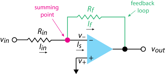
Figure \(\PageIndex{1}\) is an example of an operational amplifier circuit with a negative feedback loop that consists of a resistor, \(R_f\), that connects the op amp's output to its input at a summing point, \(S\). Because the feedback loop is connected to the op amp's inverting input, the effect is called negative feedback.
We can analyze this circuit using the laws of electricity from Chapter 2. Let's begin by rearranging Equation \ref{prop1} to solve for \(v_{out}\)
\[v_{out} = - A_{op} \times (v_{-} - v_{+}) \label{negfb0} \]
and then expand the right side of this equation
\[v_{out} = -A_{op} \times (v_{-} - v_{+}) = -A_{op} \times v_{-} + A_{op} \times v_{+} \label{negfb1} \]
and solve for \(v_{-}\)
\[v_{-} = v_{+} - \frac{v_{out}}{A_{op}} \label{negfb2} \]
Because the op amp's gain \(A_{op}\) is so large—recall that it is typically in the range 104 and 106—we can simplify Equation \ref{negfb2} to
\[v_{-} \approx v_{+} \label{negfb3} \]
One consequence of Equation \ref{negfb3} is that for this circuit \(v_{-} \approx 0 \text{ V}\) as it is at the circuit common.
From Kirchoff's laws, we know that the total current that enters the summing point must equal the total current that leaves the summing point, or
\[I_{in} = I_s + I_f \label{negfb4} \]
where \(I_s\) is the current between the op amp's two inputs. As we noted in Chapter 3.1, an operational amplifier's internal circuitry is designed such at \(I_s \approx 0\); thus
\[I_{in} = I_f \label{negfb5} \]
Substituting in Ohm's law (\(V = I \times R\)) gives
\[\frac{v_{in} - v_{-}}{R_{in}} = \frac{v_{-} - v_{out}}{R_f} \label{negfb6} \]
From Equation \ref{negfb3}, we know that \(v_{-} \approx 0\), which allows us to simplify Equation \ref{negfb6} to
\[\frac{v_{in}}{R_{in}} = -\frac{v_{out}}{R_f} \label{negfb7} \]
Rearranging, we find that the gain for the circuit, \(A_c\), is
\[A_c = \frac{v_{out}}{v_{in}} = - \frac{R_f}{R_{in}} \label{negfb8} \]
Equation \ref{negfb8} shows us that circuit in Figure \(\PageIndex{1}\) returns a voltage, \(v_{out}\), that has the opposite sign of \(v_{in}\) with a gain for the circuit that depends on only the relative values of the two resistors, \(R_f\) and \(R_{in}\).
The Voltage-Follower Circuit
Figure \(\PageIndex{2}\) shows another operational amplifier with a feedback loop. In this case the input to the op amp, \(v_{in}\), is made to the noninverting lead and the output is feed back into the op amp's inverting lead.
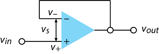
From Kirchoff's voltage law, we know that the op amp's output voltage is equal to the sum of the input voltage and the difference, \(v_s\) between the voltage applied to the op amp's two leads; thus
\[V_{out} = v_{in} + v_{s} \label{follow1} \]
The op amp's gain, \(A_{op}\), is defined in terms of \(v_s\) and \(v_{out}\)
\[- A_{op} = \frac{v_{out}}{v_{s}} \label{follow2} \]
where the minus sign is due to the change in sign between the output voltage and the voltage applied to the inverting lead. Substituting Equation \ref{follow2} into Equation \ref{follow1} gives
\[V_{in} - \frac{V_{out}}{A_{op}} = V_{out} \label{follow3} \]
Because the operational amplifier's gain—which is not the same thing as the circuit's gain—is large, Equation \ref{follow3} becomes
\[v_{in} = v_{out} \label{follow4} \]
Our analysis of this circuit shows that it returns the original voltage without any gain. It does, however, allow us to draw that voltage from the circuit with more current than the original voltage source might be able to handle.