11.6: Using R for a Principal Component Analysis
- Page ID
- 293732

\( \newcommand{\vecs}[1]{\overset { \scriptstyle \rightharpoonup} {\mathbf{#1}} } \)
\( \newcommand{\vecd}[1]{\overset{-\!-\!\rightharpoonup}{\vphantom{a}\smash {#1}}} \)
\( \newcommand{\id}{\mathrm{id}}\) \( \newcommand{\Span}{\mathrm{span}}\)
( \newcommand{\kernel}{\mathrm{null}\,}\) \( \newcommand{\range}{\mathrm{range}\,}\)
\( \newcommand{\RealPart}{\mathrm{Re}}\) \( \newcommand{\ImaginaryPart}{\mathrm{Im}}\)
\( \newcommand{\Argument}{\mathrm{Arg}}\) \( \newcommand{\norm}[1]{\| #1 \|}\)
\( \newcommand{\inner}[2]{\langle #1, #2 \rangle}\)
\( \newcommand{\Span}{\mathrm{span}}\)
\( \newcommand{\id}{\mathrm{id}}\)
\( \newcommand{\Span}{\mathrm{span}}\)
\( \newcommand{\kernel}{\mathrm{null}\,}\)
\( \newcommand{\range}{\mathrm{range}\,}\)
\( \newcommand{\RealPart}{\mathrm{Re}}\)
\( \newcommand{\ImaginaryPart}{\mathrm{Im}}\)
\( \newcommand{\Argument}{\mathrm{Arg}}\)
\( \newcommand{\norm}[1]{\| #1 \|}\)
\( \newcommand{\inner}[2]{\langle #1, #2 \rangle}\)
\( \newcommand{\Span}{\mathrm{span}}\) \( \newcommand{\AA}{\unicode[.8,0]{x212B}}\)
\( \newcommand{\vectorA}[1]{\vec{#1}} % arrow\)
\( \newcommand{\vectorAt}[1]{\vec{\text{#1}}} % arrow\)
\( \newcommand{\vectorB}[1]{\overset { \scriptstyle \rightharpoonup} {\mathbf{#1}} } \)
\( \newcommand{\vectorC}[1]{\textbf{#1}} \)
\( \newcommand{\vectorD}[1]{\overrightarrow{#1}} \)
\( \newcommand{\vectorDt}[1]{\overrightarrow{\text{#1}}} \)
\( \newcommand{\vectE}[1]{\overset{-\!-\!\rightharpoonup}{\vphantom{a}\smash{\mathbf {#1}}}} \)
\( \newcommand{\vecs}[1]{\overset { \scriptstyle \rightharpoonup} {\mathbf{#1}} } \)
\( \newcommand{\vecd}[1]{\overset{-\!-\!\rightharpoonup}{\vphantom{a}\smash {#1}}} \)
\(\newcommand{\avec}{\mathbf a}\) \(\newcommand{\bvec}{\mathbf b}\) \(\newcommand{\cvec}{\mathbf c}\) \(\newcommand{\dvec}{\mathbf d}\) \(\newcommand{\dtil}{\widetilde{\mathbf d}}\) \(\newcommand{\evec}{\mathbf e}\) \(\newcommand{\fvec}{\mathbf f}\) \(\newcommand{\nvec}{\mathbf n}\) \(\newcommand{\pvec}{\mathbf p}\) \(\newcommand{\qvec}{\mathbf q}\) \(\newcommand{\svec}{\mathbf s}\) \(\newcommand{\tvec}{\mathbf t}\) \(\newcommand{\uvec}{\mathbf u}\) \(\newcommand{\vvec}{\mathbf v}\) \(\newcommand{\wvec}{\mathbf w}\) \(\newcommand{\xvec}{\mathbf x}\) \(\newcommand{\yvec}{\mathbf y}\) \(\newcommand{\zvec}{\mathbf z}\) \(\newcommand{\rvec}{\mathbf r}\) \(\newcommand{\mvec}{\mathbf m}\) \(\newcommand{\zerovec}{\mathbf 0}\) \(\newcommand{\onevec}{\mathbf 1}\) \(\newcommand{\real}{\mathbb R}\) \(\newcommand{\twovec}[2]{\left[\begin{array}{r}#1 \\ #2 \end{array}\right]}\) \(\newcommand{\ctwovec}[2]{\left[\begin{array}{c}#1 \\ #2 \end{array}\right]}\) \(\newcommand{\threevec}[3]{\left[\begin{array}{r}#1 \\ #2 \\ #3 \end{array}\right]}\) \(\newcommand{\cthreevec}[3]{\left[\begin{array}{c}#1 \\ #2 \\ #3 \end{array}\right]}\) \(\newcommand{\fourvec}[4]{\left[\begin{array}{r}#1 \\ #2 \\ #3 \\ #4 \end{array}\right]}\) \(\newcommand{\cfourvec}[4]{\left[\begin{array}{c}#1 \\ #2 \\ #3 \\ #4 \end{array}\right]}\) \(\newcommand{\fivevec}[5]{\left[\begin{array}{r}#1 \\ #2 \\ #3 \\ #4 \\ #5 \\ \end{array}\right]}\) \(\newcommand{\cfivevec}[5]{\left[\begin{array}{c}#1 \\ #2 \\ #3 \\ #4 \\ #5 \\ \end{array}\right]}\) \(\newcommand{\mattwo}[4]{\left[\begin{array}{rr}#1 \amp #2 \\ #3 \amp #4 \\ \end{array}\right]}\) \(\newcommand{\laspan}[1]{\text{Span}\{#1\}}\) \(\newcommand{\bcal}{\cal B}\) \(\newcommand{\ccal}{\cal C}\) \(\newcommand{\scal}{\cal S}\) \(\newcommand{\wcal}{\cal W}\) \(\newcommand{\ecal}{\cal E}\) \(\newcommand{\coords}[2]{\left\{#1\right\}_{#2}}\) \(\newcommand{\gray}[1]{\color{gray}{#1}}\) \(\newcommand{\lgray}[1]{\color{lightgray}{#1}}\) \(\newcommand{\rank}{\operatorname{rank}}\) \(\newcommand{\row}{\text{Row}}\) \(\newcommand{\col}{\text{Col}}\) \(\renewcommand{\row}{\text{Row}}\) \(\newcommand{\nul}{\text{Nul}}\) \(\newcommand{\var}{\text{Var}}\) \(\newcommand{\corr}{\text{corr}}\) \(\newcommand{\len}[1]{\left|#1\right|}\) \(\newcommand{\bbar}{\overline{\bvec}}\) \(\newcommand{\bhat}{\widehat{\bvec}}\) \(\newcommand{\bperp}{\bvec^\perp}\) \(\newcommand{\xhat}{\widehat{\xvec}}\) \(\newcommand{\vhat}{\widehat{\vvec}}\) \(\newcommand{\uhat}{\widehat{\uvec}}\) \(\newcommand{\what}{\widehat{\wvec}}\) \(\newcommand{\Sighat}{\widehat{\Sigma}}\) \(\newcommand{\lt}{<}\) \(\newcommand{\gt}{>}\) \(\newcommand{\amp}{&}\) \(\definecolor{fillinmathshade}{gray}{0.9}\)To illustrate how we can use R to complete a cluster analysis: use this link and save the file allSpec.csv to your working directory. The data in this file consists of 80 rows and 642 columns. Each row is an independent sample that contains one or more of the following transition metal cations: Cu2+, Co2+, Cr3+, and Ni2+. The first seven columns provide information about the samples:
- a sample id (in the form custd_1 for a single standard of Cu2+ or nicu_mix1 for a mixture of Ni2+ and Cu2+)
- a list of the analytes in the sample (in the form cuco for a sample that contains Cu2+ and Co2+)
- the number of analytes in the sample (a number from 1 to 4 and labeled as dimensions)
- the molar concentration of Cu2+ in the sample
- the molar concentration of Co2+ in the sample
- the molar concentration of Cr3+ in the sample
- the molar concentration of Ni2+ in the sample
The remaining columns contain absorbance values at 635 wavelengths between 380.5 nm and 899.5 nm.
First, we need to read the data into R, which we do using the read.csv() function
spec_data <- read.csv("allSpec.csv", check.names = FALSE)
where the option check.names = FALSE overrides the function's default to not allow a column's name to begin with a number. Next, we will create a subset of this large data set to work with
wavelength_ids = seq(8, 642, 40)

sample_ids = c(1, 6, 11, 21:25, 38:53)

pca_data = spec_data[sample_ids, wavelength_ids ]
where wavelength_ids is a vector that identifies the 16 equally spaced wavelengths, sample_ids is a vector that identifies the 24 samples that contain one or more of the cations Cu2+, Co2+, and Cr3+, and cluster_data is a data frame that contains the absorbance values for these 24 samples at these 16 wavelengths.
To complete the principal component analysis we will use R's prcomp() function, which takes the general form
prcomp(object, center, scale)
where object is a data frame or matrix that contains our data, and center and scale are logical values that indicate if we should first center and scale the data before we complete the analysis. When we center and scale our data each variable (in this case, the absorbance at each wavelength) is adjusted so that its mean is zero and its variance is one. This has the effect of placing all variables on a common scale, which ensures that any difference in the relative magnitude of the variables does not affect the principal component analysis.
pca_results = prcomp(pca_data, center = TRUE, scale = TRUE)
The prcomp() function returns a variety of information that we can use to examine the results, including the standard deviation for each principal component, sdev, a matrix with the loadings, rotation, a matrix with the scores, x, and the values use to center and scale the original data. The summary() function, for example, returns the standard deviations for and the proportion of the overall variance explained by each principal component, and the cumulative proportion of variance explained by the principal components.
summary(pca_results)
Importance of components:
PC1 PC2 PC3 PC4 PC5 PC6 PC7 PC8 PC9
Standard deviation 3.3134 2.1901 0.42561 0.17585 0.09384 0.04607 0.04026 0.01253 0.01049
Proportion of Variance 0.6862 0.2998 0.01132 0.00193 0.00055 0.00013 0.00010 0.00001 0.00001
Cumulative Proportion 0.6862 0.9859 0.99725 0.99919 0.99974 0.99987 0.99997 0.99998 0.99999
PC10 PC11 PC12 PC13 PC14 PC15 PC16
Standard deviation 0.009211 0.007084 0.004478 0.00416 0.003039 0.002377 0.001504
Proportion of Variance 0.000010 0.000000 0.000000 0.00000 0.000000 0.000000 0.000000
Cumulative Proportion 0.999990 1.000000 1.000000 1.00000 1.000000 1.000000 1.000000
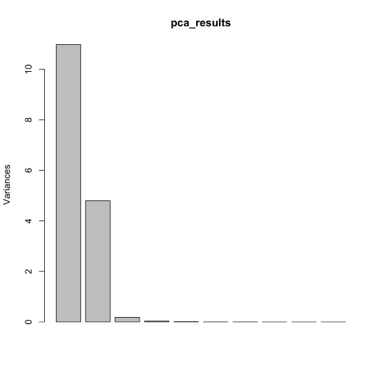
We can also examine each principal component's variance (the square of its standard deviation) in the form of a bar plot by passing the results of the principal component analysis to the plot() function.
plot(pca_results)
As noted above, the 24 samples include one, two, or three of the cations Cu2+, Co2+, and Cr3+, which is consistent with our results if individual solutions are made by combining together aliquots of stock solutions of Cu2+, Co2+, and Cr3+ and diluting to a common volume. In this case, the volume of stock solution for one cation places limits on the volumes of the other cations such that a three-component mixture essentially has two independent variables.
To examine the scores for the principal component analysis, we pass the scores to the plot() function, here using pch = 19 to display them as filled points.
plot(pca_results$x, pch = 19)
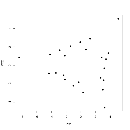
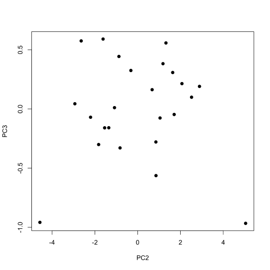
By default, the plot() function displays the values for the first two principal components, with the first (PC1) placed on the x-axis and the second (PC2) placed on the y-axis. If we wish to examine other principal components, then we must specify them when calling the plot() function; the following command, for example, uses the scores for the second and the third principal components.
plot(x = pca_results$x[,2], y = pca_results$x[,3], pch = 19, xlab = "PC2", ylab = "PC3")
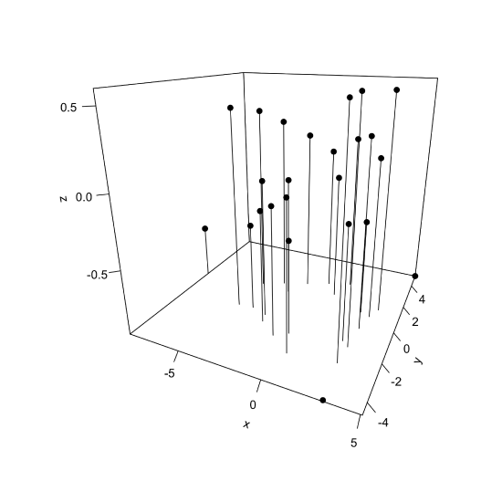
If we wish to display the first three principal components using the same plot, then we can use the scatter3D() function from the plot3D package, which takes the general form
library(plot3D)

scatter3D(x = pca_results$x[,1], y = pca_results$x[,2], z = pca_results$x[,3], pch = 19, type = "h", theta = 25, phi = 20, ticktype = "detailed", colvar = NULL)
where we use the library() function to load the package into our R session (note: this assumes you have installed the plot3D package). The option type = "h" drops a horizontal line from each point down to the plane for PC1 and PC2, which helps us orient the points in space. By default, the plot uses color to show each points value of the third principal component (displayed on the z-axis); here we set colvar = NULL to display all points using the same color.
Although the plots are not not shown here, we can use the same commands, replacing x with rotation, to display the loadings.
plot(pca_results$rotation, pch = 19)
plot(x = pca_results$rotation[,2], y = pca_results$rotation[,3], pch = 19, xlab = "PC2", ylab = "PC3")
scatter3D(x = pca_results$rotation[,1], y = pca_results$rotation[,2], z = pca_results$rotation[,3], pch = 19, type = "h", theta = 25, phi = 20, ticktype = "detailed", colvar = NULL)
Another way to view the results of a principal component analysis is to display the scores and the loadings on the same plot, which we can do using the biplot() function.
biplot(pca_results, cex = c(2, 0.6), xlabs = rep("•", 24))
where the option xlabs = rep("•", 24) overrides the function's default to display the scores as numbers, replacing them with dots, and cex = c(2, 0.6) is used to increase the size of the dots and decrease the size of the labels for the loadings.
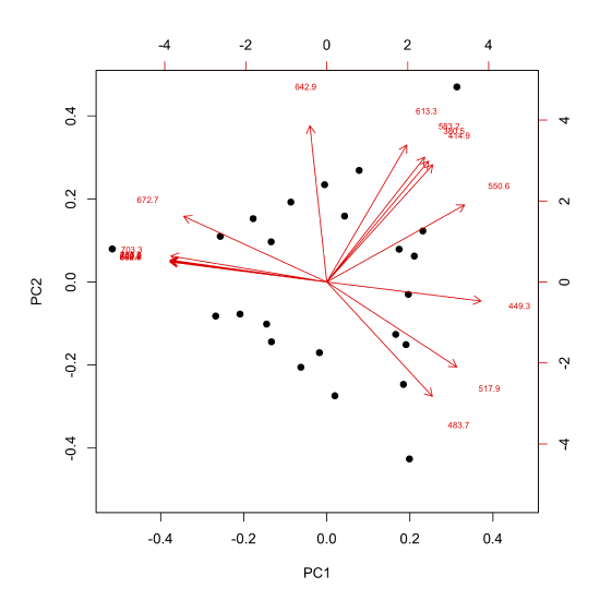
In this biplot, the scores are displayed as dots and the loadings are displayed as arrows that begin at the origin and point toward the individual loadings, which are indicated by the wavelengths associated with the loadings. For this set of data, scores and loadings that are co-located with each other represent samples and wavelengths that are strongly correlated with each other. For example, the sample whose score is in the upper right corner is strongly associated with absorbance of light with wavelengths of 613.3 nm, 583.2 nm, 380.5 nm, and 414.9 nm.
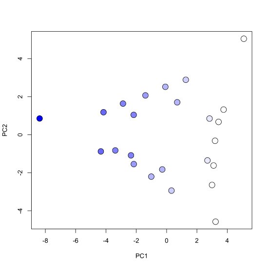
Finally, we can use use color to highlight features from our data set. For example, the following lines of code creates a scores plot that uses a color pallet to indicate the relative concentration of Cu2+ in the sample.
cu_palette = colorRampPalette(c("white", "blue"))

cu_color = cu_pallete(50)[as.numeric(cut(spec_data$concCu[sample_ids], breaks = 50))]
The colorRampPalette() function takes a vector of colors—in this case white and blue—and returns a function that we can use to create a palette of colors that runs from pure white to pure blue. We then use this function to create 50 shades of white and blue
cu_palette(50)
[1] "#FFFFFF" "#F9F9FF" "#F4F4FF" "#EFEFFF" "#EAEAFF" "#E4E4FF" "#DFDFFF" "#DADAFF"
[9] "#D5D5FF" "#D0D0FF" "#CACAFF" "#C5C5FF" "#C0C0FF" "#BBBBFF" "#B6B6FF" "#B0B0FF"
[17] "#ABABFF" "#A6A6FF" "#A1A1FF" "#9C9CFF" "#9696FF" "#9191FF" "#8C8CFF" "#8787FF"
[25] "#8282FF" "#7C7CFF" "#7777FF" "#7272FF" "#6D6DFF" "#6868FF" "#6262FF" "#5D5DFF"
[33] "#5858FF" "#5353FF" "#4E4EFF" "#4848FF" "#4343FF" "#3E3EFF" "#3939FF" "#3434FF"
[41] "#2E2EFF" "#2929FF" "#2424FF" "#1F1FFF" "#1A1AFF" "#1414FF" "#0F0FFF" "#0A0AFF"
[49] "#0505FF" "#0000FF"
where #FFFFFF is the hexadecimal code for pure white and #0000FF is the hexadecimal code for pure blue. The latter part of this line of code
cu_color = cu_pallete(50)[as.numeric(cut(spec_data$concCu[sample_ids], breaks = 50))]
retrieves the concentrations of copper in each of our 24 samples and assigns a hexadecimal code for a shade of blue that indicates the relative concentration of copper in the sample. Here we see that the first sample has a hexadecimal code of #0000FF for pure blue, which means this sample has the largest concentration of copper and samples 2–8 have hexademical codes of #FFFFFF for pure white, which means these samples do not contain any copper.
cu_color
[1] "#0000FF" "#FFFFFF" "#FFFFFF" "#FFFFFF" "#FFFFFF" "#FFFFFF" "#FFFFFF" "#FFFFFF"
[9] "#D0D0FF" "#B6B6FF" "#9C9CFF" "#8282FF" "#6868FF" "#D0D0FF" "#B6B6FF" "#9C9CFF"
[17] "#8282FF" "#6868FF" "#EAEAFF" "#EAEAFF" "#B6B6FF" "#B6B6FF" "#8282FF" "#8282FF"
Finally, we create the scores plot, using pch = 21 for an open circle whose background color we designate using bg = cu_color and where we use cex = 2 to increase the size of the points.
plot(pca_results$x, pch = 21, bg = cu_color, cex = 2)