11.5: Using R for a Cluster Analysis
- Page ID
- 293730

\( \newcommand{\vecs}[1]{\overset { \scriptstyle \rightharpoonup} {\mathbf{#1}} } \)
\( \newcommand{\vecd}[1]{\overset{-\!-\!\rightharpoonup}{\vphantom{a}\smash {#1}}} \)
\( \newcommand{\id}{\mathrm{id}}\) \( \newcommand{\Span}{\mathrm{span}}\)
( \newcommand{\kernel}{\mathrm{null}\,}\) \( \newcommand{\range}{\mathrm{range}\,}\)
\( \newcommand{\RealPart}{\mathrm{Re}}\) \( \newcommand{\ImaginaryPart}{\mathrm{Im}}\)
\( \newcommand{\Argument}{\mathrm{Arg}}\) \( \newcommand{\norm}[1]{\| #1 \|}\)
\( \newcommand{\inner}[2]{\langle #1, #2 \rangle}\)
\( \newcommand{\Span}{\mathrm{span}}\)
\( \newcommand{\id}{\mathrm{id}}\)
\( \newcommand{\Span}{\mathrm{span}}\)
\( \newcommand{\kernel}{\mathrm{null}\,}\)
\( \newcommand{\range}{\mathrm{range}\,}\)
\( \newcommand{\RealPart}{\mathrm{Re}}\)
\( \newcommand{\ImaginaryPart}{\mathrm{Im}}\)
\( \newcommand{\Argument}{\mathrm{Arg}}\)
\( \newcommand{\norm}[1]{\| #1 \|}\)
\( \newcommand{\inner}[2]{\langle #1, #2 \rangle}\)
\( \newcommand{\Span}{\mathrm{span}}\) \( \newcommand{\AA}{\unicode[.8,0]{x212B}}\)
\( \newcommand{\vectorA}[1]{\vec{#1}} % arrow\)
\( \newcommand{\vectorAt}[1]{\vec{\text{#1}}} % arrow\)
\( \newcommand{\vectorB}[1]{\overset { \scriptstyle \rightharpoonup} {\mathbf{#1}} } \)
\( \newcommand{\vectorC}[1]{\textbf{#1}} \)
\( \newcommand{\vectorD}[1]{\overrightarrow{#1}} \)
\( \newcommand{\vectorDt}[1]{\overrightarrow{\text{#1}}} \)
\( \newcommand{\vectE}[1]{\overset{-\!-\!\rightharpoonup}{\vphantom{a}\smash{\mathbf {#1}}}} \)
\( \newcommand{\vecs}[1]{\overset { \scriptstyle \rightharpoonup} {\mathbf{#1}} } \)
\( \newcommand{\vecd}[1]{\overset{-\!-\!\rightharpoonup}{\vphantom{a}\smash {#1}}} \)
\(\newcommand{\avec}{\mathbf a}\) \(\newcommand{\bvec}{\mathbf b}\) \(\newcommand{\cvec}{\mathbf c}\) \(\newcommand{\dvec}{\mathbf d}\) \(\newcommand{\dtil}{\widetilde{\mathbf d}}\) \(\newcommand{\evec}{\mathbf e}\) \(\newcommand{\fvec}{\mathbf f}\) \(\newcommand{\nvec}{\mathbf n}\) \(\newcommand{\pvec}{\mathbf p}\) \(\newcommand{\qvec}{\mathbf q}\) \(\newcommand{\svec}{\mathbf s}\) \(\newcommand{\tvec}{\mathbf t}\) \(\newcommand{\uvec}{\mathbf u}\) \(\newcommand{\vvec}{\mathbf v}\) \(\newcommand{\wvec}{\mathbf w}\) \(\newcommand{\xvec}{\mathbf x}\) \(\newcommand{\yvec}{\mathbf y}\) \(\newcommand{\zvec}{\mathbf z}\) \(\newcommand{\rvec}{\mathbf r}\) \(\newcommand{\mvec}{\mathbf m}\) \(\newcommand{\zerovec}{\mathbf 0}\) \(\newcommand{\onevec}{\mathbf 1}\) \(\newcommand{\real}{\mathbb R}\) \(\newcommand{\twovec}[2]{\left[\begin{array}{r}#1 \\ #2 \end{array}\right]}\) \(\newcommand{\ctwovec}[2]{\left[\begin{array}{c}#1 \\ #2 \end{array}\right]}\) \(\newcommand{\threevec}[3]{\left[\begin{array}{r}#1 \\ #2 \\ #3 \end{array}\right]}\) \(\newcommand{\cthreevec}[3]{\left[\begin{array}{c}#1 \\ #2 \\ #3 \end{array}\right]}\) \(\newcommand{\fourvec}[4]{\left[\begin{array}{r}#1 \\ #2 \\ #3 \\ #4 \end{array}\right]}\) \(\newcommand{\cfourvec}[4]{\left[\begin{array}{c}#1 \\ #2 \\ #3 \\ #4 \end{array}\right]}\) \(\newcommand{\fivevec}[5]{\left[\begin{array}{r}#1 \\ #2 \\ #3 \\ #4 \\ #5 \\ \end{array}\right]}\) \(\newcommand{\cfivevec}[5]{\left[\begin{array}{c}#1 \\ #2 \\ #3 \\ #4 \\ #5 \\ \end{array}\right]}\) \(\newcommand{\mattwo}[4]{\left[\begin{array}{rr}#1 \amp #2 \\ #3 \amp #4 \\ \end{array}\right]}\) \(\newcommand{\laspan}[1]{\text{Span}\{#1\}}\) \(\newcommand{\bcal}{\cal B}\) \(\newcommand{\ccal}{\cal C}\) \(\newcommand{\scal}{\cal S}\) \(\newcommand{\wcal}{\cal W}\) \(\newcommand{\ecal}{\cal E}\) \(\newcommand{\coords}[2]{\left\{#1\right\}_{#2}}\) \(\newcommand{\gray}[1]{\color{gray}{#1}}\) \(\newcommand{\lgray}[1]{\color{lightgray}{#1}}\) \(\newcommand{\rank}{\operatorname{rank}}\) \(\newcommand{\row}{\text{Row}}\) \(\newcommand{\col}{\text{Col}}\) \(\renewcommand{\row}{\text{Row}}\) \(\newcommand{\nul}{\text{Nul}}\) \(\newcommand{\var}{\text{Var}}\) \(\newcommand{\corr}{\text{corr}}\) \(\newcommand{\len}[1]{\left|#1\right|}\) \(\newcommand{\bbar}{\overline{\bvec}}\) \(\newcommand{\bhat}{\widehat{\bvec}}\) \(\newcommand{\bperp}{\bvec^\perp}\) \(\newcommand{\xhat}{\widehat{\xvec}}\) \(\newcommand{\vhat}{\widehat{\vvec}}\) \(\newcommand{\uhat}{\widehat{\uvec}}\) \(\newcommand{\what}{\widehat{\wvec}}\) \(\newcommand{\Sighat}{\widehat{\Sigma}}\) \(\newcommand{\lt}{<}\) \(\newcommand{\gt}{>}\) \(\newcommand{\amp}{&}\) \(\definecolor{fillinmathshade}{gray}{0.9}\)To illustrate how we can use R to complete a cluster analysis: use this link and save the file allSpec.csv to your working directory. The data in this file consists of 80 rows and 642 columns. Each row is an independent sample that contains one or more of the following transition metal cations: Cu2+, Co2+, Cr3+, and Ni2+. The first seven columns provide information about the samples:
- a sample id (in the form custd_1 for a single standard of Cu2+ or nicu_mix1 for a mixture of Ni2+ and Cu2+)
- a list of the analytes in the sample (in the form cuco for a sample that contains Cu2+ and Co2+)
- the number of analytes in the sample (a number from 1 to 4 and labeled as dimensions)
- the molar concentration of Cu2+ in the sample
- the molar concentration of Co2+ in the sample
- the molar concentration of Cr3+ in the sample
- the molar concentration of Ni2+ in the sample
The remaining columns contain absorbance values at 635 wavelengths between 380.5 nm and 899.5 nm.
First, we need to read the data into R, which we do using the read.csv() function
spec_data <- read.csv("allSpec.csv", check.names = FALSE)
where the option check.names = FALSE overrides the function's default to not allow a column's name to begin with a number. Next, we will create a subset of this large data set to work with
wavelength_ids = seq(8, 642, 40)

sample_ids = c(1, 6, 11, 21:25, 38:53)

cluster_data = spec_data[sample_ids, wavelength_ids ]
where wavelength_ids is a vector that identifies the 16 equally spaced wavelengths, sample_ids is a vector that identifies the 24 samples that contain one or more of the cations Cu2+, Co2+, and Cr3+, and cluster_data is a data frame that contains the absorbance values for these 24 samples at these 16 wavelengths.
Before we can complete the cluster analysis, we first must calculate the distance between the \(24 \times 16 = 384\) points that make up our data. To do this, we use the dist() function, which takes the general form
dist(object, method)
where object is a data frame or matrix with our data. There are a number of options for method, but we will use the default, which is euclidean.
cluster_dist = dist(cluster_data, method = "euclidean")

cluster_dist
1 6 11 21 22 23 24 25
6 1.53328104
11 1.73128979 0.96493008
21 1.48359716 0.24997370 0.77766228
22 1.49208058 0.32863786 0.68852029 0.09664215
23 1.49457333 0.42903074 0.57495499 0.21089686 0.11755129
24 1.51211374 0.52218072 0.47457024 0.31016429 0.21830998 0.10205547
25 1.55862311 0.61154277 0.39798649 0.39406580 0.30194838 0.19121251 0.09771283
38 1.17069314 0.38098750 0.96982420 0.34254297 0.38830178 0.45418483 0.53114050 0.61729900
Only a small portion of the values in cluster_dist are shown here; each entry shows the distance between two of the 24 samples.
With distances calculated, we can use R's hclust() function to complete the cluster analysis. The general form of the function is
hclust(object, method)
where object is the output created using dist() that contains the distances between points. There are a number of options for method—here we use the ward.D method—saving the output to the object cluster_results so that we have access to the results.
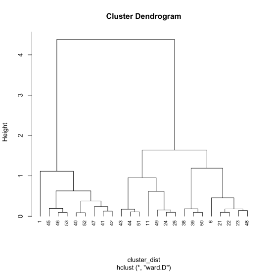
cluster_results = hclust(cluster_dist, method = "ward.D")
To view the cluster diagram, we pass the object cluster_results to the plot() function where hang = -1 extends each vertical line to a height of zero. By default, the labels at the bottom of the dendrogram are the sample ids; cex adjusts the size of these labels.
plot(cluster_results, hang = -1, cex = 0.75)
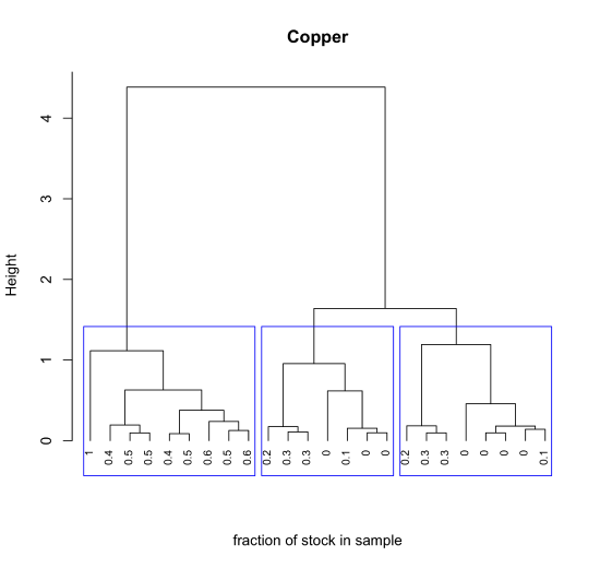
With a few lines of code we can add useful details to our plot. Here, for example, we determine the the fraction of the stock Cu2+ solution in each sample and use these values as labels, and divide the 24 samples into three large clusters using the rect.clust() function where k is the number of clusters to highlight and which indicates which of these clusters to display using a rectangular box.
cluster_copper = spec_data$concCu/spec_data$concCu[1]

plot(cluster_results, hang = -1, labels = cluster_copper[sample_ids], main = "Copper", xlab = "fraction of stock in sample", sub = "", cex = 0.75)

rect.hclust(cluster_results, k = 3, which = c(1,2,3), border = "blue")
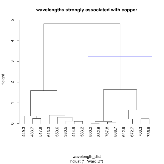
The following code shows how we can use the same data set of 24 samples and 16 wavelength to complete a cluster diagram for the wavelengths. The use of the t() function within the dist() function takes the transpose of our data so that the rows are the 16 wavelengths and the columns are the 24 samples. We do this because the dist() function calculates distances using the rows.
wavelength_dist = dist(t(cluster_data))

wavelength_clust = hclust(wavelength_dist, method = "ward.D")

plot(wavelength_clust, hang = -1, main = "wavelengths strongly associated with copper")

rect.hclust(wavelength_clust, k = 2, which = 2, border = "blue")
The figure below highlights the cluster of wavelengths most strongly associated with the absorption by Cu2+.