10.2: Improving the Signal-to-Noise Ratio

In this section we will consider three common computational tools for improving the signal-to-noise ratio: signal averaging, digital smoothing, and Fourier filtering.

Signal Averaging

The most important difference between the signal and the noise is that a signal is determinate (fixed in value) and the noise is indeterminate (random in value). If we measure a pure signal several times, we expect its value to be the same each time; thus, if we add together n scans, we expect that the net signal, \(S_n\), is defined as

\[S_n = n S \nonumber\]

where \(S\) is the signal for a single scan. Because noise is random, its value varies from one run to the next, sometimes with a value that is larger and sometimes with a value that is smaller, and sometimes with a value that is positive and sometimes with a value that is negative. On average, the standard deviation of the noise increases as we make more scans, but it does so at a slower rate than for the signal

\[s_n = \sqrt{n} s \nonumber \]

where \(s\) is the standard deviation for a single scan and \(s_n\) is the standard deviation after n scans. Combining these two equations, shows us that the signal-to-noise ratio, \(S/N\), after n scans increases as

\[(S/N)_n = \frac{S_n}{s_n} = \frac{nS}{\sqrt{n}s} = \sqrt{n}(S/N)_{n = 1} \nonumber\]

where \((S/N)_{n = 1}\) is the signal-to-noise ratio for the initial scan. Thus, when \(n = 4\) the signal-to-noise ratio improves by a factor of 2, and when \(n = 16\) the signal-to-noise ratio increases by a factor of 4. Figure \(\PageIndex{1}\) shows the improvement in the signal-to-noise ratio for 1, 2, 4, and 8 scans.

Figure \(\PageIndex{1}\): Improvement in the signal-to-noise ratio through signal averaging using 1, 2, 4, and 8 scans. Each plot shows the noisy signal in blue with the pure signal superimposed in black. The total signal is divided by the number of scans so that each y-axis has the same scale.

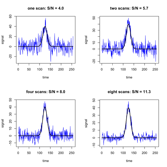
Signal averaging works well when the time it takes to collect a single scan is short and when the analyte's signal is stable with respect to time both because the sample is stable and the instrument is stable; when this is not the case, then we risk a time-dependent change in \(S_\text{analyte}\) and/or \(s_\text{noise}\) Because the equation for \((S/N)_n\) is proportional to the \(\sqrt{n}\), the relative improvement in the signal-to-noise ratio decreases as \(n\) increases; for example, 16 scans gives a \(4 \times\) improvement in the signal-to-noise ratio, but it takes an additional 48 scans (for a total of 64 scans) to achieve a \(8 \times\) improvement in the signal-to-noise ratio.

Digital Smoothing Filters

One characteristic of noise is that its magnitude fluctuates rapidly in contrast to the underlying signal. We see this, for example, in Figure \(\PageIndex{1}\) where the underlying signal either remains constant or steadily increases or decreases while the noise fluctuates chaotically. Digital smoothing filters take advantage of this by using a mathematical function to average the data for a small range of consecutive data points, replacing the range's middle value with the average signal over that range.

Moving Average Filters

For a moving average filter, we replace each point by the average signal for that point and an equal number of points on either side; thus, a moving average filtee has a width, \(w\), of 3, 5, 7, ... points. For example, suppose the first five points in a sequence are

0.80

0.30

0.80

0.20

1.00

then a three-point moving average (\(w = 3)\) returns values of

NA

0.63

0.43

0.67

NA

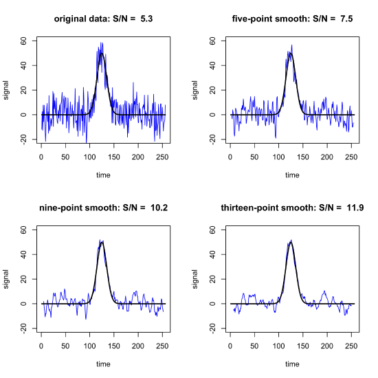
where, for example, 0.63 is the average of 0.80, 0.30, and 0.80. Note that we lose \((w - 1)/2 = (3 - 1)/2 = 1\) points at each end of the data set because we do not have a sufficient number of data points to complete a calculation for the first and the last point. Figure \(\PageIndex{2}\) shows the improvement in the \(S/N\) ratio when using moving average filters with widths of 5, 9, and 13.

Figure \(\PageIndex{2}\): Improvement in the signal-to-noise ratio using moving average filters with ranges of 5, 9, and 13 on the original data shown in the upper left quadrant. Each plot shows the noisy signal in blue with the pure signal superimposed in black.

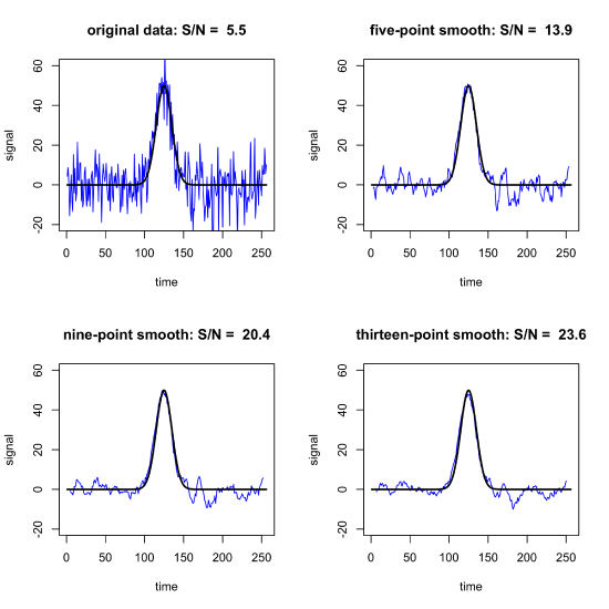
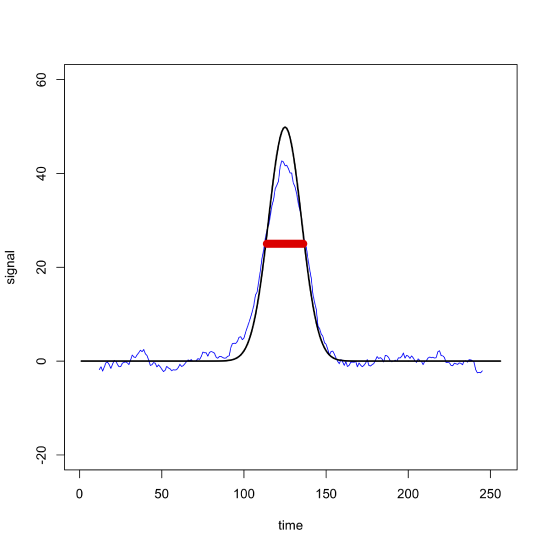
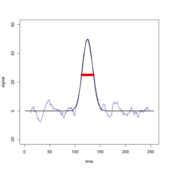
One limitation to a moving average filter is that it distorts the original data by removing points from both ends, although this is not a serious concern if the points in question are just noise. Of greater concern is the distortion in a signal's height if we use a range that is too wide; for example, Figure \(\PageIndex{3}\), shows how a 23-point moving average filter (shown in blue) applied to the noisy signal in the upper left quadrant of Figure \(\PageIndex{2}\), reduces the height of the original signal (shown in black). Because the filter's width—shown by the red bar—is similar to the peak's width, as the filter passes through the peak it systematically reduces the signal by averaging together values that are mostly smaller than the maximum signal.

Figure \(\PageIndex{3}\): Example that shows how a moving average filter can distort the signal when applied to the noisy signal in the upper left quadrant of Figure \(\PageIndex{2}\). The original pure signal is shown in black and the signal after applying a 23-point moving average filter is shown in blue. The width of the moving average filter is shown by the red bar.

Savitzky-Golay Filters

A moving average filter weights all points equally; that is, points near the edges of the filter contribute to the average as a level equal to points near the filter's center. A Savitzky-Golay filter uses a polynomial model that weights each point differently, placing more weight on points near the center of the filter and less weight on points at the edge of the filter. Specific values depend on the size of the window and the polynomial model; for example, a five-point filter using a second-order polynomial has weights of

\[-3/35 \quad \quad 12/35 \quad \quad 17/35 \quad \quad 12/35 \quad \quad -3/35 \nonumber \]

For example, suppose the first five points in a sequence are

0.80

0.30

0.80

0.20

1.00

then this Savitzky-Golay filter returns values of

NA

NA

0.41

NA

NA

where, for example, the value for the middle point is

\[0.80 \times \frac{-3}{35} + 0.30 \times \frac{12}{35} + 0.80 \times \frac{17}{35} + 0.20 \times \frac{12}{35} + 1.00 \times \frac{-3}{35} = 0.406 \approx 0.41 \nonumber \]

Note that we lose \((w - 1)/2 = (5 - 1)/2 = 2\) points at each end of the data set, where w is the filter's range, because we do not have a sufficient number of data points to complete the calculations. For other Savitzky-Golay smoothing filters, see Savitzky, A.; Golay, M. J. E. Anal Chem, 1964, 36, 1627-1639. Figure \(\PageIndex{4}\) shows the improvement in the \(S/N\) ratio when using Savitzky-Golay filters using a second-order polynomial with 5, 9, and 13 points.

Figure \(\PageIndex{4}\): Improvement in the signal-to-noise ratio using Savitzky-Golay filters of ranges of 5, 9, and 13 on the original data shown in the upper left quadrant. Each plot shows the noisy signal in blue with the pure signal superimposed in black.

Because a Savitzky-Golay filter weights points differently than does a moving average smoothing filter, a Savitzky-Golay filter introduces less distortion to the signal, as we see in the following figure.

Figure \(\PageIndex{5}\): A Savitzky-Golay filter is less aggressive than a moving average filter. Applying a 23-point Savitzky-Golay filter to the noisy signal in the upper left quadrant of Figure \(\PageIndex{4}\) results in little distortion of the signal. Contrast this with Figure \(\PageIndex{3}\) where a 23-point moving average filter results in substantial distortion of the signal. The original pure signal is shown in black and the signal after applying a 23-point Savitzky-Golay filter is shown in blue. The width of the Savitzky-Golay filter is shown by the red bar.

Fourier Filtering

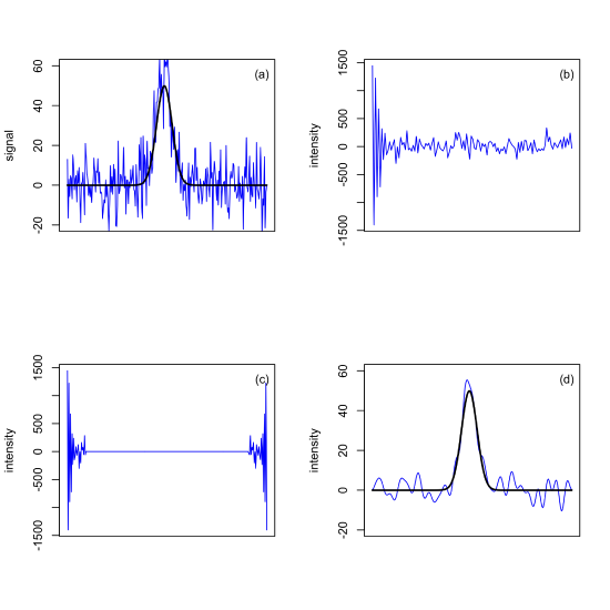
This approach to improving the signal-to-noise ratio takes advantage of a mathematical technique called a Fourier transform (FT). The basis of a Fourier transform is that we can express a signal in two separate domains. In the first domain the signal is characterized by one or more peaks, each defined by its position, its width, and its area; this is called the frequency domain. In the second domain, which is called the time domain, the signal consists of a set of oscillations, each defined by its frequency, its amplitude, and its decay rate. The Fourier transform—and the inverse Fourier transform—allow us to move between these two domains.

Note

The mathematical details behind the Fourier transform are beyond the level of this textbook; for a more in-depth treatment, consult this chapter's resources.

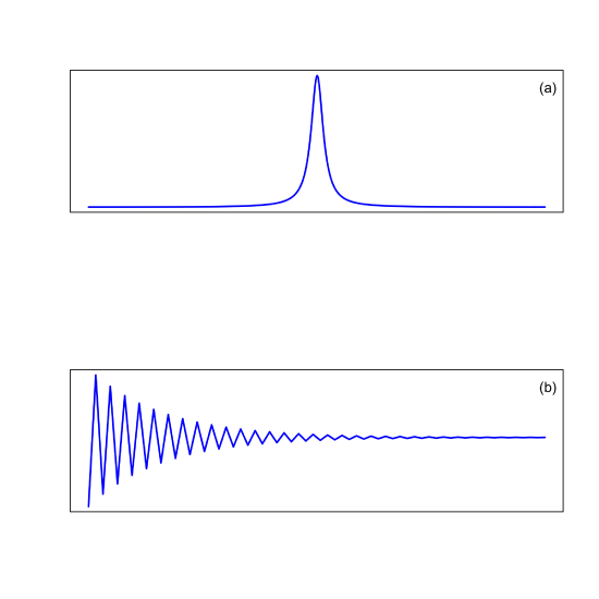
Figure \(\PageIndex{6a}\) shows a single peak in the frequency domain and Figure \(\PageIndex{6b}\) shows its equivalent time domain signal. There are correlations between the two domains:

• the further a peak in the frequency domain is from the origin, the greater it corresponding oscillation frequency in the time domain
• the broader a peak's width in the frequency domain, the faster its decay rate in the time domain
• the greater the area under a peak in the frequency domain, the higher its initial intensity in the time domain

Figure \(\PageIndex{6}\): The plot in (a) shows a frequency domain consisting of a single peak defined by its position along the x-axis, its width, and its area. The plot in (b) shows the corresponding time domain that consists of a single oscillating signal defined by its oscillation frequency, its initial intensity, and its decay rate.

We can use a Fourier transform to improve the signal-to-noise ratio because the signal is a single broad peak and the noise appears as a multitude of very narrow peaks. As noted above, a broad peak in the frequency domain has a fast decaying signal in the time domain, which means that while the beginning of the time domain signal includes contributions from the signal and the noise, the latter part of the time domain signal includes contributions from noise only. The figure below shows how we can take advantage of this to reduce the noise and improve the signal-to-noise ratio for the noisy signal in Figure \(\PageIndex{7a}\), which has 256 points along the x-axis and has a signal-to-noise ratio of 5.1. First, we use the Fourier transform to convert its original domain into the new domain, the first 128 points of which are shown in Figure \(\PageIndex{7b}\) (note: the first half of the data contains the same information as the second half of the data, so we only need to look at the first half of the data). The points at the beginning are dominated by the signal, which is why there is a systematic decrease in the intensity of the oscillations; the remaining points are dominated by noise, which is why the variation in intensity is random. To filter out the noise we retain the first 24 points as they are and set the intensities of the remaining points to zero (the choice of how many points to retain may require some adjustment). As shown in Figure \(\PageIndex{7c}\), we repeat this for the remaining 128 points, retaining the last 24 points as they are. Finally, we use an inverse Fourier transform to return to our original domain, with the result in Figure \(\PageIndex{7d}\), with the signal-to-noise ratio improving from 5. 1 for the original noisy signal to 11.2 for the filtered signal.

Figure \(\PageIndex{7}\): Example of removing noise using a Fourier filter. The original noisy signal with \(S/N = 5.1\) is shown in (a) and is similar to the noisy signal in Figure \(\PageIndex{2a}\) and Figure \(\PageIndex{4a}\). The first half of the Fourier transformed data is shown in (b). The Fourier transformed data is shown in (c) after zeroing out all but the first and the last 24 points. Returning to the original domain gives the final filtered signal with \(S/N = 11.1\).