10.1: Signals and Noise

When we make a measurement it is the sum of two parts, a determinate, or fixed contribution that arises from the analyte and an indeterminate, or random, contribution that arises from uncertainty in the measurement process. We call the first of these the signal and we call the latter the noise. There are two broad categories of noise: that associated with obtaining samples and that associated with making measurements. Our interest here is in the latter.

What is Noise?

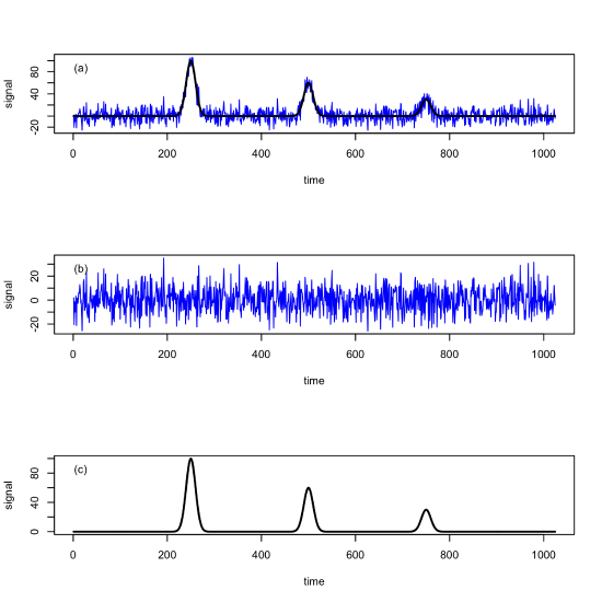
Noise is a random event characterized by a mean and standard deviation. There are many types of noise, but we will limit ourselves for now to noise that is stationary, in that its mean and its standard deviation are independent of time, and that is heteroscedastic, in that its mean and its variance (and standard deviation) are independent of the signal's magnitude. Figure \(\PageIndex{1a}\) shows an example of a noisy signal that meets these criteria. The x-axis here is shown as time—perhaps a chromatogram—but other units, such as wavelength or potential, are possible. Figure \(\PageIndex{1b}\) shows the underlying noise and Figure \(\PageIndex{1c}\) shows the underlying signal. Note that the noise in Figure \(\PageIndex{1b}\) appears consistent in its central tendency (mean) and its spread (variance) along the x-axis and is independent of the signal's strength.

Figure \(\PageIndex{1}\): Plots showing (a) the signal and the noise in blue with the signal superimposed as a smooth line; (b) the noise only; and (c) the signal only. The signal consists of three peaks at times of 250, 500, and 750, and with maximum values of 100, 60, and 30, respectively. The noise is drawn at random from a normal distribution with a mean of 0 and a standard deviation of 10.

How Do We Characterize the Signal and the Noise?

Although we characterize noise by its mean and its standard deviation, the most important benchmark is the signal-to-noise ratio, \(S/N\), which we define as

\[S/N = \frac{S_\text{analyte}}{s_\text{noise}} \nonumber\]

where \(S_\text{analyte}\) is the signal's value at particular location on the x-axis and \(s_\text{noise}\) is the standard deviation of the noise using a signal-free portion of the data. As general rules-of-thumb, we can measure the signal with some confidence when \(S/N \ge 3\) and we can detect the signal with some confidence when \(3 \ge S/N \ge 2\). For the data in Figure \(\PageIndex{1}\), and using the information in the figure caption, the signal-to-noise ratios are, from left-to-right, 10, 6, and 3.

Note

To measure the signal with confidence implies we can use the signal's value in a calculation, such as constructing a calibration curve. To detect the signal with confidence means we are certain that a signal is present (and that an analyte responsible for the signal is present) even if we cannot measure the signal with sufficient confidence to allow for a meaningful calculation.

How Can We Improve the \(S/N\) Ratio?

There are two broad approaches that we can use to improve the signal-to-noise ratio: hardware and software. Hardware approaches are built into the instrument and include decisions on how the instrument is set-up for making measurements (for example, the choice of a scan rate or a slit width), and how the signal is processed by the instrument (for example, using electronic filters); such solutions are not of interest to us here in a textbook with a focus on chemometrics. Software solutions are computational approaches in which we manipulate the data either while we are collecting it or after data acquisition is complete.