8.2: Weighted Linear Regression with Errors in y

Last updated
Save as PDF

Page ID: 290632

\( \newcommand{\vecs}[1]{\overset { \scriptstyle \rightharpoonup} {\mathbf{#1}} } \) \( \newcommand{\vecd}[1]{\overset{-\!-\!\rightharpoonup}{\vphantom{a}\smash {#1}}} \)\(\newcommand{\id}{\mathrm{id}}\) \( \newcommand{\Span}{\mathrm{span}}\) \( \newcommand{\kernel}{\mathrm{null}\,}\) \( \newcommand{\range}{\mathrm{range}\,}\) \( \newcommand{\RealPart}{\mathrm{Re}}\) \( \newcommand{\ImaginaryPart}{\mathrm{Im}}\) \( \newcommand{\Argument}{\mathrm{Arg}}\) \( \newcommand{\norm}[1]{\| #1 \|}\) \( \newcommand{\inner}[2]{\langle #1, #2 \rangle}\) \( \newcommand{\Span}{\mathrm{span}}\) \(\newcommand{\id}{\mathrm{id}}\) \( \newcommand{\Span}{\mathrm{span}}\) \( \newcommand{\kernel}{\mathrm{null}\,}\) \( \newcommand{\range}{\mathrm{range}\,}\) \( \newcommand{\RealPart}{\mathrm{Re}}\) \( \newcommand{\ImaginaryPart}{\mathrm{Im}}\) \( \newcommand{\Argument}{\mathrm{Arg}}\) \( \newcommand{\norm}[1]{\| #1 \|}\) \( \newcommand{\inner}[2]{\langle #1, #2 \rangle}\) \( \newcommand{\Span}{\mathrm{span}}\)\(\newcommand{\AA}{\unicode[.8,0]{x212B}}\)

Our treatment of linear regression to this point assumes that any indeterminate errors that affect y are independent of the value of x. If this assumption is false, then we must include the variance for each value of y in our determination of the y-intercept, b₀, and the slope, b₁; thus

\[b_0 = \frac {\sum_{i = 1}^{n} w_i y_i - b_1 \sum_{i = 1}^{n} w_i x_i} {n} \nonumber \]

\[b_1 = \frac {n \sum_{i = 1}^{n} w_i x_i y_i - \sum_{i = 1}^{n} w_i x_i \sum_{i = 1}^{n} w_i y_i} {n \sum_{i =1}^{n} w_i x_i^2 - \left( \sum_{i = 1}^{n} w_i x_i \right)^2} \nonumber\]

where w_i is a weighting factor that accounts for the variance in y_i

\[w_i = \frac {n (s_{y_i})^{-2}} {\sum_{i = 1}^{n} (s_{y_i})^{-2}} \nonumber\]

and \(s_{y_i}\) is the standard deviation for y_i. In a weighted linear regression, each xy-pair’s contribution to the regression line is inversely proportional to the precision of y_i; that is, the more precise the value of y, the greater its contribution to the regression.

Example \(\PageIndex{4}\)

Shown here are data for an external standardization in which s_std is the standard deviation for three replicate determination of the signal. This is the same data used in the examples in Section 8.1 with additional information about the standard deviations in the signal.

\(C_{std}\) (arbitrary units)	\(S_{std}\) (arbitrary units)	\(s_{std}\)
0.000	0.00	0.02
0.100	12.36	0.02
0.200	24.83	0.07
0.300	35.91	0.13
0.400	48.79	0.22
0.500	60.42	0.33

Determine the calibration curve’s equation using a weighted linear regression. As you work through this example, remember that x corresponds to C_std, and that y corresponds to S_std.

Solution

We begin by setting up a table to aid in calculating the weighting factors.

\(C_{std}\) (arbitrary units)	\(S_{std}\) (arbitrary units)	\(s_{std}\)	\((s_{y_i})^{-2}\)	\(w_i\)
0.000	0.00	0.02	2500.00	2.8339
0.100	12.36	0.02	250.00	2.8339
0.200	24.83	0.07	204.08	0.2313
0.300	35.91	0.13	59.17	0.0671
0.400	48.79	0.22	20.66	0.0234
0.500	60.42	0.33	9.18	0.0104

Adding together the values in the fourth column gives

\[\sum_{i = 1}^{n} (s_{y_i})^{-2} \nonumber\]

which we use to calculate the individual weights in the last column. As a check on your calculations, the sum of the individual weights must equal the number of calibration standards, n. The sum of the entries in the last column is 6.0000, so all is well. After we calculate the individual weights, we use a second table to aid in calculating the four summation terms in the equations for the slope, \(b_1\), and the y-intercept, \(b_0\).

\(x_i\)	\(y_i\)	\(w_i\)	\(w_i x_i\)	\(w_i y_i\)	\(w_i x_i^2\)	\(w_i x_i y_i\)
0.000	0.00	2.8339	0.0000	0.0000	0.0000	0.0000
0.100	12.36	2.8339	0.2834	35.0270	0.0283	3.5027
0.200	24.83	0.2313	0.0463	5.7432	0.0093	1.1486
0.300	35.91	0.0671	0.0201	2.4096	0.0060	0.7229
0.400	48.79	0.0234	0.0094	1.1417	0.0037	0.4567
0.500	60.42	0.0104	0.0052	0.6284	0.0026	0.3142

Adding the values in the last four columns gives

\[\sum_{i = 1}^{n} w_i x_i = 0.3644 \quad \sum_{i = 1}^{n} w_i y_i = 44.9499 \quad \sum_{i = 1}^{n} w_i x_i^2 = 0.0499 \quad \sum_{i = 1}^{n} w_i x_i y_i = 6.1451 \nonumber\]

which gives the estimated slope and the estimated y-intercept as

\[b_1 = \frac {(6 \times 6.1451) - (0.3644 \times 44.9499)} {(6 \times 0.0499) - (0.3644)^2} = 122.985 \nonumber\]

\[b_0 = \frac{44.9499 - (122.985 \times 0.3644)} {6} = 0.0224 \nonumber\]

The calibration equation is

\[S_{std} = 122.98 \times C_{std} + 0.2 \nonumber\]

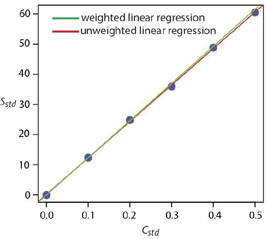
Figure \(\PageIndex{1}\) shows the calibration curve for the weighted regression determined here and the calibration curve for the unweighted regression in from Section 8.2. Although the two calibration curves are very similar, there are slight differences in the slope and in the y-intercept. Most notably, the y-intercept for the weighted linear regression is closer to the expected value of zero. Because the standard deviation for the signal, S_std, is smaller for smaller concentrations of analyte, C_std, a weighted linear regression gives more emphasis to these standards, allowing for a better estimate of the y-intercept.

Figure5.14.png — Figure \(\PageIndex{1}\): A comparison of the unweighted and the weighted normal calibration curves. See Example \(\PageIndex{1}\) for details of the unweighted linear regression and Example \(\PageIndex{4}\) for details of the weighted linear regression.

Equations for calculating confidence intervals for the slope, the y-intercept, and the concentration of analyte when using a weighted linear regression are not as easy to define as for an unweighted linear regression [Bonate, P. J. Anal. Chem. 1993, 65, 1367–1372]. The confidence interval for the analyte’s concentration, however, is at its optimum value when the analyte’s signal is near the weighted centroid, y_c , of the calibration curve.

\[y_c = \frac {1} {n} \sum_{i = 1}^{n} w_i x_i \nonumber\]