8.1: Unweighted Linear Regression With Errors in y
- Page ID
- 290597
\( \newcommand{\vecs}[1]{\overset { \scriptstyle \rightharpoonup} {\mathbf{#1}} } \)
\( \newcommand{\vecd}[1]{\overset{-\!-\!\rightharpoonup}{\vphantom{a}\smash {#1}}} \)
\( \newcommand{\id}{\mathrm{id}}\) \( \newcommand{\Span}{\mathrm{span}}\)
( \newcommand{\kernel}{\mathrm{null}\,}\) \( \newcommand{\range}{\mathrm{range}\,}\)
\( \newcommand{\RealPart}{\mathrm{Re}}\) \( \newcommand{\ImaginaryPart}{\mathrm{Im}}\)
\( \newcommand{\Argument}{\mathrm{Arg}}\) \( \newcommand{\norm}[1]{\| #1 \|}\)
\( \newcommand{\inner}[2]{\langle #1, #2 \rangle}\)
\( \newcommand{\Span}{\mathrm{span}}\)
\( \newcommand{\id}{\mathrm{id}}\)
\( \newcommand{\Span}{\mathrm{span}}\)
\( \newcommand{\kernel}{\mathrm{null}\,}\)
\( \newcommand{\range}{\mathrm{range}\,}\)
\( \newcommand{\RealPart}{\mathrm{Re}}\)
\( \newcommand{\ImaginaryPart}{\mathrm{Im}}\)
\( \newcommand{\Argument}{\mathrm{Arg}}\)
\( \newcommand{\norm}[1]{\| #1 \|}\)
\( \newcommand{\inner}[2]{\langle #1, #2 \rangle}\)
\( \newcommand{\Span}{\mathrm{span}}\) \( \newcommand{\AA}{\unicode[.8,0]{x212B}}\)
\( \newcommand{\vectorA}[1]{\vec{#1}} % arrow\)
\( \newcommand{\vectorAt}[1]{\vec{\text{#1}}} % arrow\)
\( \newcommand{\vectorB}[1]{\overset { \scriptstyle \rightharpoonup} {\mathbf{#1}} } \)
\( \newcommand{\vectorC}[1]{\textbf{#1}} \)
\( \newcommand{\vectorD}[1]{\overrightarrow{#1}} \)
\( \newcommand{\vectorDt}[1]{\overrightarrow{\text{#1}}} \)
\( \newcommand{\vectE}[1]{\overset{-\!-\!\rightharpoonup}{\vphantom{a}\smash{\mathbf {#1}}}} \)
\( \newcommand{\vecs}[1]{\overset { \scriptstyle \rightharpoonup} {\mathbf{#1}} } \)
\( \newcommand{\vecd}[1]{\overset{-\!-\!\rightharpoonup}{\vphantom{a}\smash {#1}}} \)
\(\newcommand{\avec}{\mathbf a}\) \(\newcommand{\bvec}{\mathbf b}\) \(\newcommand{\cvec}{\mathbf c}\) \(\newcommand{\dvec}{\mathbf d}\) \(\newcommand{\dtil}{\widetilde{\mathbf d}}\) \(\newcommand{\evec}{\mathbf e}\) \(\newcommand{\fvec}{\mathbf f}\) \(\newcommand{\nvec}{\mathbf n}\) \(\newcommand{\pvec}{\mathbf p}\) \(\newcommand{\qvec}{\mathbf q}\) \(\newcommand{\svec}{\mathbf s}\) \(\newcommand{\tvec}{\mathbf t}\) \(\newcommand{\uvec}{\mathbf u}\) \(\newcommand{\vvec}{\mathbf v}\) \(\newcommand{\wvec}{\mathbf w}\) \(\newcommand{\xvec}{\mathbf x}\) \(\newcommand{\yvec}{\mathbf y}\) \(\newcommand{\zvec}{\mathbf z}\) \(\newcommand{\rvec}{\mathbf r}\) \(\newcommand{\mvec}{\mathbf m}\) \(\newcommand{\zerovec}{\mathbf 0}\) \(\newcommand{\onevec}{\mathbf 1}\) \(\newcommand{\real}{\mathbb R}\) \(\newcommand{\twovec}[2]{\left[\begin{array}{r}#1 \\ #2 \end{array}\right]}\) \(\newcommand{\ctwovec}[2]{\left[\begin{array}{c}#1 \\ #2 \end{array}\right]}\) \(\newcommand{\threevec}[3]{\left[\begin{array}{r}#1 \\ #2 \\ #3 \end{array}\right]}\) \(\newcommand{\cthreevec}[3]{\left[\begin{array}{c}#1 \\ #2 \\ #3 \end{array}\right]}\) \(\newcommand{\fourvec}[4]{\left[\begin{array}{r}#1 \\ #2 \\ #3 \\ #4 \end{array}\right]}\) \(\newcommand{\cfourvec}[4]{\left[\begin{array}{c}#1 \\ #2 \\ #3 \\ #4 \end{array}\right]}\) \(\newcommand{\fivevec}[5]{\left[\begin{array}{r}#1 \\ #2 \\ #3 \\ #4 \\ #5 \\ \end{array}\right]}\) \(\newcommand{\cfivevec}[5]{\left[\begin{array}{c}#1 \\ #2 \\ #3 \\ #4 \\ #5 \\ \end{array}\right]}\) \(\newcommand{\mattwo}[4]{\left[\begin{array}{rr}#1 \amp #2 \\ #3 \amp #4 \\ \end{array}\right]}\) \(\newcommand{\laspan}[1]{\text{Span}\{#1\}}\) \(\newcommand{\bcal}{\cal B}\) \(\newcommand{\ccal}{\cal C}\) \(\newcommand{\scal}{\cal S}\) \(\newcommand{\wcal}{\cal W}\) \(\newcommand{\ecal}{\cal E}\) \(\newcommand{\coords}[2]{\left\{#1\right\}_{#2}}\) \(\newcommand{\gray}[1]{\color{gray}{#1}}\) \(\newcommand{\lgray}[1]{\color{lightgray}{#1}}\) \(\newcommand{\rank}{\operatorname{rank}}\) \(\newcommand{\row}{\text{Row}}\) \(\newcommand{\col}{\text{Col}}\) \(\renewcommand{\row}{\text{Row}}\) \(\newcommand{\nul}{\text{Nul}}\) \(\newcommand{\var}{\text{Var}}\) \(\newcommand{\corr}{\text{corr}}\) \(\newcommand{\len}[1]{\left|#1\right|}\) \(\newcommand{\bbar}{\overline{\bvec}}\) \(\newcommand{\bhat}{\widehat{\bvec}}\) \(\newcommand{\bperp}{\bvec^\perp}\) \(\newcommand{\xhat}{\widehat{\xvec}}\) \(\newcommand{\vhat}{\widehat{\vvec}}\) \(\newcommand{\uhat}{\widehat{\uvec}}\) \(\newcommand{\what}{\widehat{\wvec}}\) \(\newcommand{\Sighat}{\widehat{\Sigma}}\) \(\newcommand{\lt}{<}\) \(\newcommand{\gt}{>}\) \(\newcommand{\amp}{&}\) \(\definecolor{fillinmathshade}{gray}{0.9}\)The most common method for completing a linear regression makes three assumptions:
- the difference between our experimental data and the calculated regression line is the result of indeterminate errors that affect y
- any indeterminate errors that affect y are normally distributed
- that indeterminate errors in y are independent of the value of x
Because we assume that the indeterminate errors are the same for all standards, each standard contributes equally in our estimate of the slope and the y-intercept. For this reason the result is considered an unweighted linear regression.
The second assumption generally is true because of the central limit theorem, which we considered in Chapter 5.3. The validity of the two remaining assumptions is less obvious and you should evaluate them before you accept the results of a linear regression. In particular the first assumption is always suspect because there certainly is some indeterminate error in the measurement of x. When we prepare a calibration curve, however, it is not unusual to find that the uncertainty in the signal, S, is significantly greater than the uncertainty in the analyte’s concentration, \(C_A\). In such circumstances the first assumption usually is reasonable.
How a Linear Regression Works
To understand the logic of a linear regression consider the example in Figure \(\PageIndex{1}\), which shows three data points and two possible straight-lines that might reasonably explain the data. How do we decide how well these straight-lines fit the data, and how do we determine which, if either, is the best straight-line?
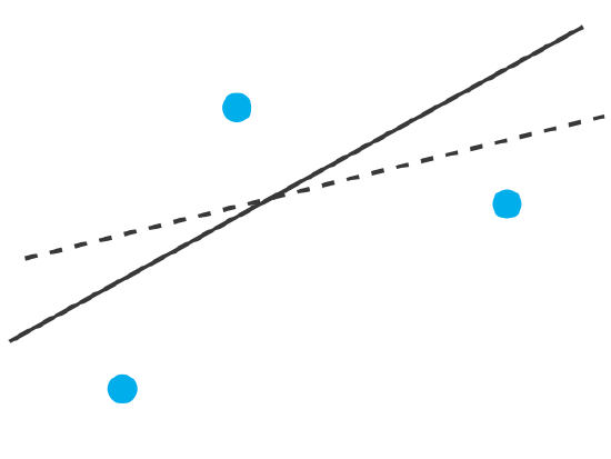
Let’s focus on the solid line in Figure \(\PageIndex{1}\). The equation for this line is
\[\hat{y} = b_0 + b_1 x \nonumber \]
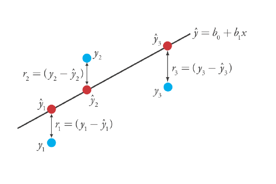
where b0 and b1 are estimates for the y-intercept and the slope, and \(\hat{y}\) is the predicted value of y for any value of x. Because we assume that all uncertainty is the result of indeterminate errors in y, the difference between y and \(\hat{y}\) for each value of x is the residual error, r, in our mathematical model.
\[r_i = (y_i - \hat{y}_i) \nonumber\]
Figure \(\PageIndex{2}\) shows the residual errors for the three data points. The smaller the total residual error, R, which we define as
\[R = \sum_{i = 1}^{n} (y_i - \hat{y}_i)^2 \nonumber \]
the better the fit between the straight-line and the data. In a linear regression analysis, we seek values of b0 and b1 that give the smallest total residual error.
The reason for squaring the individual residual errors is to prevent a positive residual error from canceling out a negative residual error. You have seen this before in the equations for the sample and population standard deviations introduced in Chapter 4. You also can see from this equation why a linear regression is sometimes called the method of least squares.
Finding the Slope and y-Intercept for the Regression Model
Although we will not formally develop the mathematical equations for a linear regression analysis, you can find the derivations in many standard statistical texts [ See, for example, Draper, N. R.; Smith, H. Applied Regression Analysis, 3rd ed.; Wiley: New York, 1998]. The resulting equation for the slope, b1, is
\[b_1 = \frac {n \sum_{i = 1}^{n} x_i y_i - \sum_{i = 1}^{n} x_i \sum_{i = 1}^{n} y_i} {n \sum_{i = 1}^{n} x_i^2 - \left( \sum_{i = 1}^{n} x_i \right)^2} \nonumber \]
and the equation for the y-intercept, b0, is
\[b_0 = \frac {\sum_{i = 1}^{n} y_i - b_1 \sum_{i = 1}^{n} x_i} {n} \nonumber \]
Although these equations appear formidable, it is necessary only to evaluate the following four summations
\[\sum_{i = 1}^{n} x_i \quad \sum_{i = 1}^{n} y_i \quad \sum_{i = 1}^{n} x_i y_i \quad \sum_{i = 1}^{n} x_i^2 \nonumber\]
Many calculators, spreadsheets, and other statistical software packages are capable of performing a linear regression analysis based on this model; see Section 8.5 for details on completing a linear regression analysis using R. For illustrative purposes the necessary calculations are shown in detail in the following example.
Using the calibration data in the following table, determine the relationship between the signal, \(y_i\), and the analyte's concentration, \(x_i\), using an unweighted linear regression.
Solution
We begin by setting up a table to help us organize the calculation.
| \(x_i\) | \(y_i\) | \(x_i y_i\) | \(x_i^2\) |
|---|---|---|---|
| 0.000 | 0.00 | 0.000 | 0.000 |
| 0.100 | 12.36 | 1.236 | 0.010 |
| 0.200 | 24.83 | 4.966 | 0.040 |
| 0.300 | 35.91 | 10.773 | 0.090 |
| 0.400 | 48.79 | 19.516 | 0.160 |
| 0.500 | 60.42 | 30.210 | 0.250 |
Adding the values in each column gives
\[\sum_{i = 1}^{n} x_i = 1.500 \quad \sum_{i = 1}^{n} y_i = 182.31 \quad \sum_{i = 1}^{n} x_i y_i = 66.701 \quad \sum_{i = 1}^{n} x_i^2 = 0.550 \nonumber\]
Substituting these values into the equations for the slope and the y-intercept gives
\[b_1 = \frac {(6 \times 66.701) - (1.500 \times 182.31)} {(6 \times 0.550) - (1.500)^2} = 120.706 \approx 120.71 \nonumber\]
\[b_0 = \frac {182.31 - (120.706 \times 1.500)} {6} = 0.209 \approx 0.21 \nonumber\]
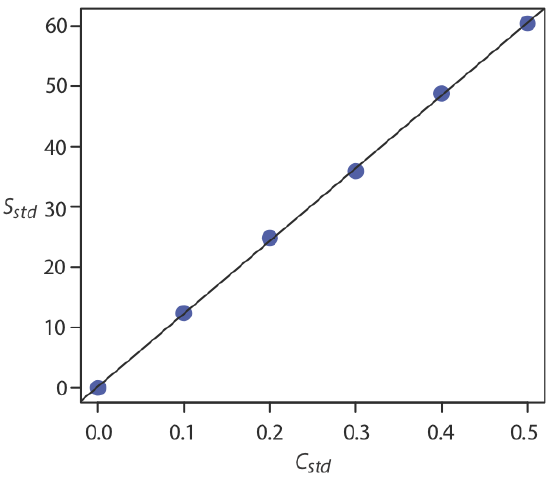
The relationship between the signal, \(S\), and the analyte's concentration, \(C_A\), therefore, is
\[S = 120.71 \times C_A + 0.21 \nonumber\]
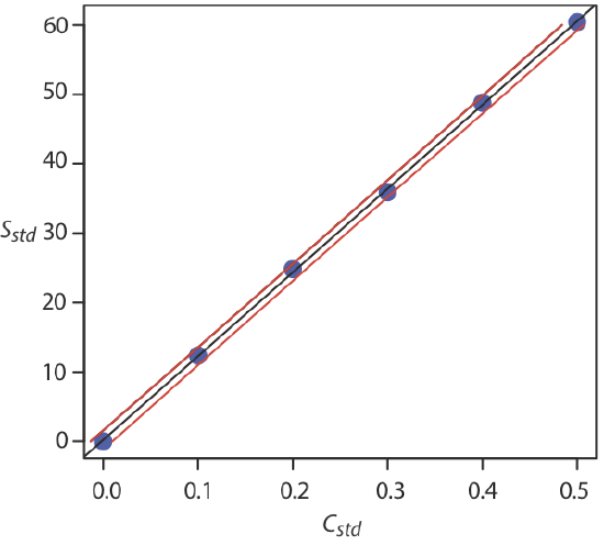
For now we keep two decimal places to match the number of decimal places in the signal. The resulting calibration curve is shown in Figure \(\PageIndex{3}\).
Uncertainty in the Regression Model
As we see in Figure \(\PageIndex{3}\), because of indeterminate errors in the signal, the regression line does not pass through the exact center of each data point. The cumulative deviation of our data from the regression line—the total residual error—is proportional to the uncertainty in the regression. We call this uncertainty the standard deviation about the regression, sr, which is equal to
\[s_r = \sqrt{\frac {\sum_{i = 1}^{n} \left( y_i - \hat{y}_i \right)^2} {n - 2}} \nonumber \]
where yi is the ith experimental value, and \(\hat{y}_i\) is the corresponding value predicted by the regression equation \(\hat{y} = b_0 + b_1 x\). Note that the denominator indicates that our regression analysis has n – 2 degrees of freedom—we lose two degree of freedom because we use two parameters, the slope and the y-intercept, to calculate \(\hat{y}_i\).
A more useful representation of the uncertainty in our regression analysis is to consider the effect of indeterminate errors on the slope, b1, and the y-intercept, b0, which we express as standard deviations.
\[s_{b_1} = \sqrt{\frac {n s_r^2} {n \sum_{i = 1}^{n} x_i^2 - \left( \sum_{i = 1}^{n} x_i \right)^2}} = \sqrt{\frac {s_r^2} {\sum_{i = 1}^{n} \left( x_i - \overline{x} \right)^2}} \nonumber \]
\[s_{b_0} = \sqrt{\frac {s_r^2 \sum_{i = 1}^{n} x_i^2} {n \sum_{i = 1}^{n} x_i^2 - \left( \sum_{i = 1}^{n} x_i \right)^2}} = \sqrt{\frac {s_r^2 \sum_{i = 1}^{n} x_i^2} {n \sum_{i = 1}^{n} \left( x_i - \overline{x} \right)^2}} \nonumber \]
We use these standard deviations to establish confidence intervals for the expected slope, \(\beta_1\), and the expected y-intercept, \(\beta_0\)
\[\beta_1 = b_1 \pm t s_{b_1} \nonumber \]
\[\beta_0 = b_0 \pm t s_{b_0} \nonumber \]
where we select t for a significance level of \(\alpha\) and for n – 2 degrees of freedom. Note that these equations do not contain the factor of \((\sqrt{n})^{-1}\) seen in the confidence intervals for \(\mu\) in Chapter 6.2; this is because the confidence interval here is based on a single regression line.
Calculate the 95% confidence intervals for the slope and y-intercept from Example \(\PageIndex{1}\).
Solution
We begin by calculating the standard deviation about the regression. To do this we must calculate the predicted signals, \(\hat{y}_i\) , using the slope and the y-intercept from Example \(\PageIndex{1}\), and the squares of the residual error, \((y_i - \hat{y}_i)^2\). Using the last standard as an example, we find that the predicted signal is
\[\hat{y}_6 = b_0 + b_1 x_6 = 0.209 + (120.706 \times 0.500) = 60.562 \nonumber\]
and that the square of the residual error is
\[(y_i - \hat{y}_i)^2 = (60.42 - 60.562)^2 = 0.2016 \approx 0.202 \nonumber\]
The following table displays the results for all six solutions.
| \(x_i\) | \(y_i\) | \(\hat{y}_i\) |
\(\left( y_i - \hat{y}_i \right)^2\) |
|---|---|---|---|
| 0.000 | 0.00 | 0.209 | 0.0437 |
| 0.100 | 12.36 | 12.280 | 0.0064 |
| 0.200 | 24.83 | 24.350 | 0.2304 |
| 0.300 | 35.91 | 36.421 | 0.2611 |
| 0.400 | 48.79 | 48.491 | 0.0894 |
| 0.500 | 60.42 | 60.562 | 0.0202 |
Adding together the data in the last column gives the numerator in the equation for the standard deviation about the regression; thus
\[s_r = \sqrt{\frac {0.6512} {6 - 2}} = 0.4035 \nonumber\]
Next we calculate the standard deviations for the slope and the y-intercept. The values for the summation terms are from Example \(\PageIndex{1}\).
\[s_{b_1} = \sqrt{\frac {6 \times (0.4035)^2} {(6 \times 0.550) - (1.500)^2}} = 0.965 \nonumber\]
\[s_{b_0} = \sqrt{\frac {(0.4035)^2 \times 0.550} {(6 \times 0.550) - (1.500)^2}} = 0.292 \nonumber\]
Finally, the 95% confidence intervals (\(\alpha = 0.05\), 4 degrees of freedom) for the slope and y-intercept are
\[\beta_1 = b_1 \pm ts_{b_1} = 120.706 \pm (2.78 \times 0.965) = 120.7 \pm 2.7 \nonumber\]
\[\beta_0 = b_0 \pm ts_{b_0} = 0.209 \pm (2.78 \times 0.292) = 0.2 \pm 0.80 \nonumber\]
where t(0.05, 4) from Appendix 2 is 2.78. The standard deviation about the regression, sr, suggests that the signal, Sstd, is precise to one decimal place. For this reason we report the slope and the y-intercept to a single decimal place.
Using the Regression Model to Determine a Value for x Given a Value for y
Once we have our regression equation, it is easy to determine the concentration of analyte in a sample. When we use a normal calibration curve, for example, we measure the signal for our sample, Ssamp, and calculate the analyte’s concentration, CA, using the regression equation.
\[C_A = \frac {S_{samp} - b_0} {b_1} \nonumber \]
What is less obvious is how to report a confidence interval for CA that expresses the uncertainty in our analysis. To calculate a confidence interval we need to know the standard deviation in the analyte’s concentration, \(s_{C_A}\), which is given by the following equation
\[s_{C_A} = \frac {s_r} {b_1} \sqrt{\frac {1} {m} + \frac {1} {n} + \frac {\left( \overline{S}_{samp} - \overline{S}_{std} \right)^2} {(b_1)^2 \sum_{i = 1}^{n} \left( C_{std_i} - \overline{C}_{std} \right)^2}} \nonumber\]
where m is the number of replicates we use to establish the sample’s average signal, Ssamp, n is the number of calibration standards, Sstd is the average signal for the calibration standards, and \(C_{std_i}\) and \(\overline{C}_{std}\) are the individual and the mean concentrations for the calibration standards. Knowing the value of \(s_{C_A}\), the confidence interval for the analyte’s concentration is
\[\mu_{C_A} = C_A \pm t s_{C_A} \nonumber\]
where \(\mu_{C_A}\) is the expected value of CA in the absence of determinate errors, and with the value of t is based on the desired level of confidence and n – 2 degrees of freedom.
A close examination of these equations should convince you that we can decrease the uncertainty in the predicted concentration of analyte, \(C_A\) if we increase the number of standards, \(n\), increase the number of replicate samples that we analyze, \(m\), and if the sample’s average signal, \(\overline{S}_{samp}\), is equal to the average signal for the standards, \(\overline{S}_{std}\). When practical, you should plan your calibration curve so that Ssamp falls in the middle of the calibration curve. For more information about these regression equations see (a) Miller, J. N. Analyst 1991, 116, 3–14; (b) Sharaf, M. A.; Illman, D. L.; Kowalski, B. R. Chemometrics, Wiley-Interscience: New York, 1986, pp. 126-127; (c) Analytical Methods Committee “Uncertainties in concentrations estimated from calibration experiments,” AMC Technical Brief, March 2006.
The equation for the standard deviation in the analyte's concentration is written in terms of a calibration experiment. A more general form of the equation, written in terms of x and y, is given here.
\[s_{x} = \frac {s_r} {b_1} \sqrt{\frac {1} {m} + \frac {1} {n} + \frac {\left( \overline{Y} - \overline{y} \right)^2} {(b_1)^2 \sum_{i = 1}^{n} \left( x_i - \overline{x} \right)^2}} \nonumber\]
Three replicate analyses for a sample that contains an unknown concentration of analyte, yields values for Ssamp of 29.32, 29.16 and 29.51 (arbitrary units). Using the results from Example \(\PageIndex{1}\) and Example \(\PageIndex{2}\), determine the analyte’s concentration, CA, and its 95% confidence interval.
Solution
The average signal, \(\overline{S}_{samp}\), is 29.33, which, using the slope and the y-intercept from Example \(\PageIndex{1}\), gives the analyte’s concentration as
\[C_A = \frac {\overline{S}_{samp} - b_0} {b_1} = \frac {29.33 - 0.209} {120.706} = 0.241 \nonumber\]
To calculate the standard deviation for the analyte’s concentration we must determine the values for \(\overline{S}_{std}\) and for \(\sum_{i = 1}^{2} (C_{std_i} - \overline{C}_{std})^2\). The former is just the average signal for the calibration standards, which, using the data in Table \(\PageIndex{1}\), is 30.385. Calculating \(\sum_{i = 1}^{2} (C_{std_i} - \overline{C}_{std})^2\) looks formidable, but we can simplify its calculation by recognizing that this sum-of-squares is the numerator in a standard deviation equation; thus,
\[\sum_{i = 1}^{n} (C_{std_i} - \overline{C}_{std})^2 = (s_{C_{std}})^2 \times (n - 1) \nonumber\]
where \(s_{C_{std}}\) is the standard deviation for the concentration of analyte in the calibration standards. Using the data in Table \(\PageIndex{1}\) we find that \(s_{C_{std}}\) is 0.1871 and
\[\sum_{i = 1}^{n} (C_{std_i} - \overline{C}_{std})^2 = (0.1872)^2 \times (6 - 1) = 0.175 \nonumber\]
Substituting known values into the equation for \(s_{C_A}\) gives
\[s_{C_A} = \frac {0.4035} {120.706} \sqrt{\frac {1} {3} + \frac {1} {6} + \frac {(29.33 - 30.385)^2} {(120.706)^2 \times 0.175}} = 0.0024 \nonumber\]
Finally, the 95% confidence interval for 4 degrees of freedom is
\[\mu_{C_A} = C_A \pm ts_{C_A} = 0.241 \pm (2.78 \times 0.0024) = 0.241 \pm 0.007 \nonumber\]
Figure \(\PageIndex{4}\) shows the calibration curve with curves showing the 95% confidence interval for CA.
Evaluating a Regression Model
You should never accept the result of a linear regression analysis without evaluating the validity of the model. Perhaps the simplest way to evaluate a regression analysis is to examine the residual errors. As we saw earlier, the residual error for a single calibration standard, ri, is
\[r_i = (y_i - \hat{y}_i) \nonumber\]
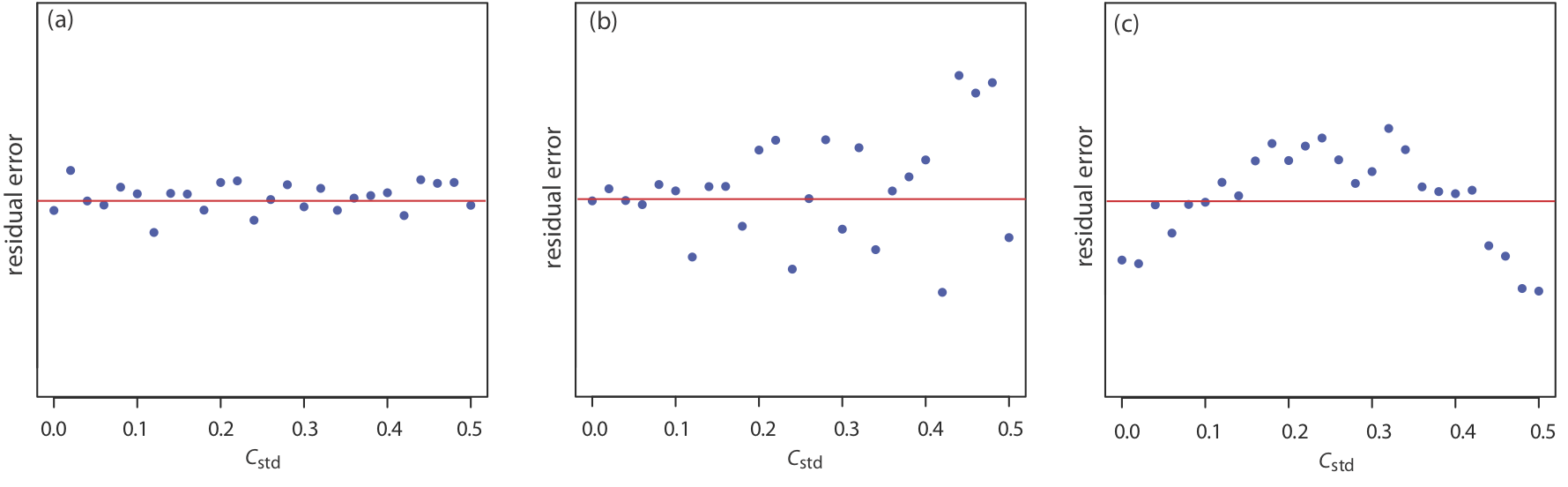
If the regression model is valid, then the residual errors should be distributed randomly about an average residual error of zero, with no apparent trend toward either smaller or larger residual errors (Figure \(\PageIndex{5a}\)). Trends such as those in Figure \(\PageIndex{5b}\) and Figure \(\PageIndex{5c}\) provide evidence that at least one of the model’s assumptions is incorrect. For example, a trend toward larger residual errors at higher concentrations, Figure \(\PageIndex{5b}\), suggests that the indeterminate errors affecting the signal are not independent of the analyte’s concentration. In Figure \(\PageIndex{5c}\), the residual errors are not random, which suggests we cannot model the data using a straight-line relationship. Regression methods for the latter two cases are discussed in the following sections.
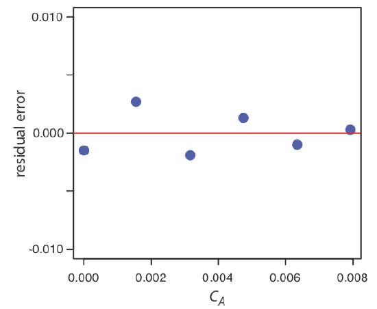
Use your results from Exercise \(\PageIndex{1}\) to construct a residual plot and explain its significance.
Solution
To create a residual plot, we need to calculate the residual error for each standard. The following table contains the relevant information.
| \(x_i\) | \(y_i\) | \(\hat{y}_i\) | \(y_i - \hat{y}_i\) |
|---|---|---|---|
| 0.000 | 0.000 | 0.0015 | –0.0015 |
| \(1.55 \times 10^{-3}\) | 0.050 | 0.0473 | 0.0027 |
| \(3.16 \times 10^{-3}\) | 0.093 | 0.0949 | –0.0019 |
| \(4.74 \times 10^{-3}\) | 0.143 | 0.1417 | 0.0013 |
| \(6.34 \times 10^{-3}\) | 0.188 | 0.1890 | –0.0010 |
| \(7.92 \times 10^{-3}\) | 0.236 | 0.2357 | 0.0003 |
The figure below shows a plot of the resulting residual errors. The residual errors appear random, although they do alternate in sign, and they do not show any significant dependence on the analyte’s concentration. Taken together, these observations suggest that our regression model is appropriate.