
6.2: Confidence Intervals
- Page ID
- 220900

In the previous section, we learned how to predict the probability of obtaining a particular outcome if our data are normally distributed with a known \(\mu\) and a known \(\sigma\). For example, we estimated that 11.60% of samples drawn at random from a standard reference material will have a concentration of Pb greater than 5.650 ppb given a \(\mu\) of 5.5833 ppb and a \(\sigma\) of 0.0558 ppb. In essence, we determined how many standard deviations 5.650 is from \(\mu\) and used this to define the probability given the standard area under a normal distribution curve.
We can look at this in a different way by asking the following question: If we collect a single sample at random from a population with a known \(\mu\) and a known \(\sigma\), within what range of values might we reasonably expect to find the sample’s result 95% of the time? Rearranging the equation
\[z = \frac {x - \mu} {\sigma} \nonumber\]
and solving for \(x\) gives
\[x = \mu \pm z \sigma = 5.5833 \pm (1.96)(0.0558) = 5.5833 \pm 0.1094 \nonumber\]
where a \(z\) of 1.96 corresponds to 95% of the area under the curve; we call this a 95% confidence interval for a single sample.
It generally is a poor idea to draw a conclusion from the result of a single experiment; instead, we usually collect several samples and ask the question this way: If we collect \(n\) random samples from a population with a known \(\mu\) and a known \(\sigma\), within what range of values might we reasonably expect to find the mean of these samples 95% of the time?
We might reasonably expect that the standard deviation for the mean of several samples is smaller than the standard deviation for a set of individual samples; indeed it is and it is given as
\[\sigma_{\bar{x}} = \frac {\sigma} {\sqrt{n}} \nonumber\]
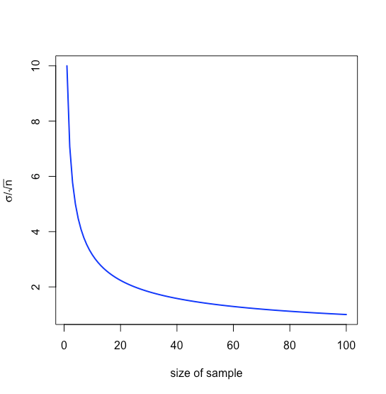
where \(\frac {\sigma} {\sqrt{n}}\) is called the standard error of the mean. For example, if we collect three samples from the standard reference material described above, then we expect that the mean for these three samples will fall within a range
\[\bar{x} = \mu \pm z \sigma_{\bar{X}} = \mu \pm \frac {z \sigma} {\sqrt{n}} = 5.5833 \pm \frac{(1.96)(0.0558)} {\sqrt{3}} = 5.5833 \pm 0.0631 \nonumber\]
that is \(\pm 0.0631\) ppb around \(\mu\), a range that is smaller than that of \(\pm 0.1094\) ppb when we analyze individual samples. Note that the relative value to us of increasing the sample’s size diminishes as \(n\) increases because of the square root term, as shown in Figure \(\PageIndex{1}\).
Our treatment thus far assumes we know \(\mu\) and \(\sigma\) for the parent population, but we rarely know these values; instead, we examine samples drawn from the parent population and ask the following question: Given the sample’s mean, \(\bar{x}\), and its standard deviation, \(s\), what is our best estimate of the population’s mean, \(\mu\), and its standard deviation, \(\sigma\).
To make this estimate, we replace the population’s standard deviation, \(\sigma\), with the standard deviation, \(s\), for our samples, replace the population’s mean, \(\mu\), with the mean, \(\bar{x}\), for our samples, replace \(z\) with \(t\), where the value of \(t\) depends on the number of samples, \(n\)
\[\bar{x} = \mu \pm \frac{ts}{\sqrt{n}} \nonumber\]
and then rearrange the equation to solve for \(\mu\).
\[\mu = \bar{x} \pm \frac {ts} {\sqrt{n}} \nonumber\]
We call this a confidence interval. Values for \(t\) are available in tables (see Appendix 2) and depend on the probability level, \(\alpha\), where \((1 − \alpha) \times 100\) is the confidence level, and the degrees of freedom, \(n − 1\); note that for any probability level, \(t \longrightarrow z\) as \(n \longrightarrow \infty\).
We need to give special attention to what this confidence interval means and to what it does not mean:
- It does not mean that there is a 95% probability that the population’s mean is in the range \(\mu = \bar{x} \pm ts\) because our measurements may be biased or the normal distribution may be inappropriate for our system.
- It does provide our best estimate of the population’s mean, \(\mu\) given our analysis of \(n\) samples drawn at random from the parent population; a different sample, however, will give a different confidence interval and, therefore, a different estimate for \(\mu\).