6.1: Properties of a Normal Distribution
- Page ID
- 220899

\( \newcommand{\vecs}[1]{\overset { \scriptstyle \rightharpoonup} {\mathbf{#1}} } \)
\( \newcommand{\vecd}[1]{\overset{-\!-\!\rightharpoonup}{\vphantom{a}\smash {#1}}} \)
\( \newcommand{\id}{\mathrm{id}}\) \( \newcommand{\Span}{\mathrm{span}}\)
( \newcommand{\kernel}{\mathrm{null}\,}\) \( \newcommand{\range}{\mathrm{range}\,}\)
\( \newcommand{\RealPart}{\mathrm{Re}}\) \( \newcommand{\ImaginaryPart}{\mathrm{Im}}\)
\( \newcommand{\Argument}{\mathrm{Arg}}\) \( \newcommand{\norm}[1]{\| #1 \|}\)
\( \newcommand{\inner}[2]{\langle #1, #2 \rangle}\)
\( \newcommand{\Span}{\mathrm{span}}\)
\( \newcommand{\id}{\mathrm{id}}\)
\( \newcommand{\Span}{\mathrm{span}}\)
\( \newcommand{\kernel}{\mathrm{null}\,}\)
\( \newcommand{\range}{\mathrm{range}\,}\)
\( \newcommand{\RealPart}{\mathrm{Re}}\)
\( \newcommand{\ImaginaryPart}{\mathrm{Im}}\)
\( \newcommand{\Argument}{\mathrm{Arg}}\)
\( \newcommand{\norm}[1]{\| #1 \|}\)
\( \newcommand{\inner}[2]{\langle #1, #2 \rangle}\)
\( \newcommand{\Span}{\mathrm{span}}\) \( \newcommand{\AA}{\unicode[.8,0]{x212B}}\)
\( \newcommand{\vectorA}[1]{\vec{#1}} % arrow\)
\( \newcommand{\vectorAt}[1]{\vec{\text{#1}}} % arrow\)
\( \newcommand{\vectorB}[1]{\overset { \scriptstyle \rightharpoonup} {\mathbf{#1}} } \)
\( \newcommand{\vectorC}[1]{\textbf{#1}} \)
\( \newcommand{\vectorD}[1]{\overrightarrow{#1}} \)
\( \newcommand{\vectorDt}[1]{\overrightarrow{\text{#1}}} \)
\( \newcommand{\vectE}[1]{\overset{-\!-\!\rightharpoonup}{\vphantom{a}\smash{\mathbf {#1}}}} \)
\( \newcommand{\vecs}[1]{\overset { \scriptstyle \rightharpoonup} {\mathbf{#1}} } \)
\( \newcommand{\vecd}[1]{\overset{-\!-\!\rightharpoonup}{\vphantom{a}\smash {#1}}} \)
\(\newcommand{\avec}{\mathbf a}\) \(\newcommand{\bvec}{\mathbf b}\) \(\newcommand{\cvec}{\mathbf c}\) \(\newcommand{\dvec}{\mathbf d}\) \(\newcommand{\dtil}{\widetilde{\mathbf d}}\) \(\newcommand{\evec}{\mathbf e}\) \(\newcommand{\fvec}{\mathbf f}\) \(\newcommand{\nvec}{\mathbf n}\) \(\newcommand{\pvec}{\mathbf p}\) \(\newcommand{\qvec}{\mathbf q}\) \(\newcommand{\svec}{\mathbf s}\) \(\newcommand{\tvec}{\mathbf t}\) \(\newcommand{\uvec}{\mathbf u}\) \(\newcommand{\vvec}{\mathbf v}\) \(\newcommand{\wvec}{\mathbf w}\) \(\newcommand{\xvec}{\mathbf x}\) \(\newcommand{\yvec}{\mathbf y}\) \(\newcommand{\zvec}{\mathbf z}\) \(\newcommand{\rvec}{\mathbf r}\) \(\newcommand{\mvec}{\mathbf m}\) \(\newcommand{\zerovec}{\mathbf 0}\) \(\newcommand{\onevec}{\mathbf 1}\) \(\newcommand{\real}{\mathbb R}\) \(\newcommand{\twovec}[2]{\left[\begin{array}{r}#1 \\ #2 \end{array}\right]}\) \(\newcommand{\ctwovec}[2]{\left[\begin{array}{c}#1 \\ #2 \end{array}\right]}\) \(\newcommand{\threevec}[3]{\left[\begin{array}{r}#1 \\ #2 \\ #3 \end{array}\right]}\) \(\newcommand{\cthreevec}[3]{\left[\begin{array}{c}#1 \\ #2 \\ #3 \end{array}\right]}\) \(\newcommand{\fourvec}[4]{\left[\begin{array}{r}#1 \\ #2 \\ #3 \\ #4 \end{array}\right]}\) \(\newcommand{\cfourvec}[4]{\left[\begin{array}{c}#1 \\ #2 \\ #3 \\ #4 \end{array}\right]}\) \(\newcommand{\fivevec}[5]{\left[\begin{array}{r}#1 \\ #2 \\ #3 \\ #4 \\ #5 \\ \end{array}\right]}\) \(\newcommand{\cfivevec}[5]{\left[\begin{array}{c}#1 \\ #2 \\ #3 \\ #4 \\ #5 \\ \end{array}\right]}\) \(\newcommand{\mattwo}[4]{\left[\begin{array}{rr}#1 \amp #2 \\ #3 \amp #4 \\ \end{array}\right]}\) \(\newcommand{\laspan}[1]{\text{Span}\{#1\}}\) \(\newcommand{\bcal}{\cal B}\) \(\newcommand{\ccal}{\cal C}\) \(\newcommand{\scal}{\cal S}\) \(\newcommand{\wcal}{\cal W}\) \(\newcommand{\ecal}{\cal E}\) \(\newcommand{\coords}[2]{\left\{#1\right\}_{#2}}\) \(\newcommand{\gray}[1]{\color{gray}{#1}}\) \(\newcommand{\lgray}[1]{\color{lightgray}{#1}}\) \(\newcommand{\rank}{\operatorname{rank}}\) \(\newcommand{\row}{\text{Row}}\) \(\newcommand{\col}{\text{Col}}\) \(\renewcommand{\row}{\text{Row}}\) \(\newcommand{\nul}{\text{Nul}}\) \(\newcommand{\var}{\text{Var}}\) \(\newcommand{\corr}{\text{corr}}\) \(\newcommand{\len}[1]{\left|#1\right|}\) \(\newcommand{\bbar}{\overline{\bvec}}\) \(\newcommand{\bhat}{\widehat{\bvec}}\) \(\newcommand{\bperp}{\bvec^\perp}\) \(\newcommand{\xhat}{\widehat{\xvec}}\) \(\newcommand{\vhat}{\widehat{\vvec}}\) \(\newcommand{\uhat}{\widehat{\uvec}}\) \(\newcommand{\what}{\widehat{\wvec}}\) \(\newcommand{\Sighat}{\widehat{\Sigma}}\) \(\newcommand{\lt}{<}\) \(\newcommand{\gt}{>}\) \(\newcommand{\amp}{&}\) \(\definecolor{fillinmathshade}{gray}{0.9}\)Mathematically a normal distribution is defined by the equation
\[P(x) = \frac {1} {\sqrt{2 \pi \sigma^2}} e^{-(x - \mu)^2/(2 \sigma^2)} \nonumber\]
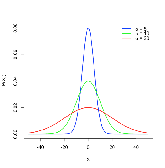
where \(P(x)\) is the probability of obtaining a result, \(x\), from a population with a known mean, \(\mu\), and a known standard deviation, \(\sigma\). Figure \(\PageIndex{1}\) shows the normal distribution curves for \(\mu = 0\) with standard deviations of 5, 10, and 20.
Because the equation for a normal distribution depends solely on the population’s mean, \(\mu\), and its standard deviation, \(\sigma\), the probability that a sample drawn from a population has a value between any two arbitrary limits is the same for all populations. For example, Figure \(\PageIndex{2}\) shows that 68.26% of all samples drawn from a normally distributed population have values within the range \(\mu \pm 1\sigma\), and only 0.14% have values greater than \(\mu + 3\sigma\).
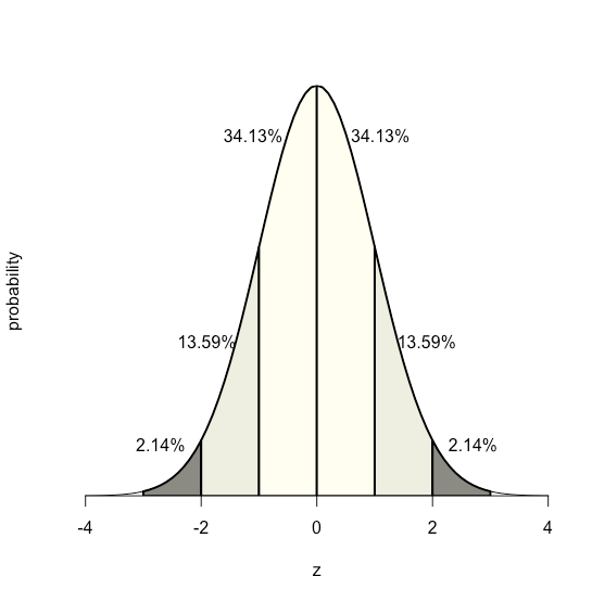
This feature of a normal distribution—that the area under the curve is the same for all values of \(\sigma\)—allows us to create a probability table (see Appendix 1) based on the relative deviation, \(z\), between a limit, x, and the mean, \(\mu\).
\[z = \frac {x - \mu} {\sigma} \nonumber\]
The value of \(z\) gives the area under the curve between that limit and the distribution’s closest tail, as shown in Figure \(\PageIndex{3}\).
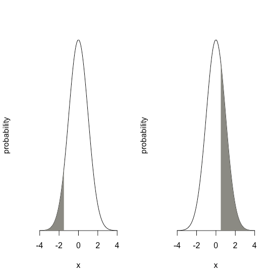
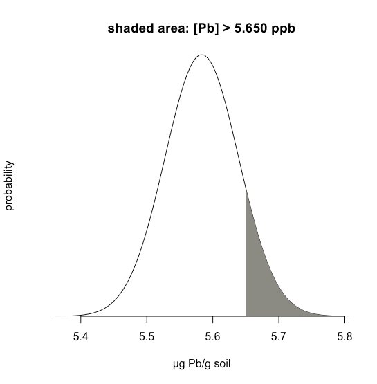
Suppose we know that \(\mu\) is 5.5833 ppb Pb and that \(\sigma\) is 0.0558 ppb Pb for a particular standard reference material (SRM). What is the probability that we will obtain a result that is greater than 5.650 ppb if we analyze a single, random sample drawn from the SRM?
Solution
Figure \(\PageIndex{4}\) shows the normal distribution curve given values of 5.5833 ppb Pb for \(\mu\) and of 0.0558 ppb Pb \(\sigma\). The shaded area in the figures is the probability of obtaining a sample with a concentration of Pb greater than 5.650 ppm. To determine the probability, we first calculate \(z\)
\[z = \frac {x - \mu} {\sigma} = \frac {5.650 - 5.5833} {0.0558} = 1.195 \nonumber\]
Next, we look up the probability in Appendix 1 for this value of \(z\), which is the average of 0.1170 (for \(z = 1.19\)) and 0.1151 (for \(z = 1.20\)), or a probability of 0.1160; thus, we expect that 11.60% of samples will provide a result greater than 5.650 ppb Pb.
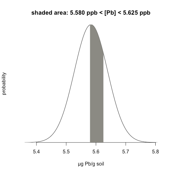
Example \(\PageIndex{1}\) considers a single limit—the probability that a result exceeds a single value. But what if we want to determine the probability that a sample has between 5.580 g Pb and 5.625 g Pb?
Solution
In this case we are interested in the shaded area shown in Figure \(\PageIndex{5}\). First, we calculate \(z\) for the upper limit
\[z = \frac {5.625 - 5.5833} {0.0558} = 0.747 \nonumber\]
and then we calculate \(z\) for the lower limit
\[z = \frac {5.580 - 5.5833} {0.0558} = -0.059 \nonumber\]
Then, we look up the probability in Appendix 1 that a result will exceed our upper limit of 5.625, which is 0.2275, or 22.75%, and the probability that a result will be less than our lower limit of 5.580, which is 0.4765, or 47.65%. The total unshaded area is 71.4% of the total area, so the shaded area corresponds to a probability of
\[100.00 - 22.75 - 47.65 = 100.00 - 71.40 = 29.6 \% \nonumber\]