
6: Self Assessment Activities- Answer Key
- Page ID
- 527190

\( \newcommand{\vecs}[1]{\overset { \scriptstyle \rightharpoonup} {\mathbf{#1}} } \)
\( \newcommand{\vecd}[1]{\overset{-\!-\!\rightharpoonup}{\vphantom{a}\smash {#1}}} \)
\( \newcommand{\dsum}{\displaystyle\sum\limits} \)
\( \newcommand{\dint}{\displaystyle\int\limits} \)
\( \newcommand{\dlim}{\displaystyle\lim\limits} \)
\( \newcommand{\id}{\mathrm{id}}\) \( \newcommand{\Span}{\mathrm{span}}\)
( \newcommand{\kernel}{\mathrm{null}\,}\) \( \newcommand{\range}{\mathrm{range}\,}\)
\( \newcommand{\RealPart}{\mathrm{Re}}\) \( \newcommand{\ImaginaryPart}{\mathrm{Im}}\)
\( \newcommand{\Argument}{\mathrm{Arg}}\) \( \newcommand{\norm}[1]{\| #1 \|}\)
\( \newcommand{\inner}[2]{\langle #1, #2 \rangle}\)
\( \newcommand{\Span}{\mathrm{span}}\)
\( \newcommand{\id}{\mathrm{id}}\)
\( \newcommand{\Span}{\mathrm{span}}\)
\( \newcommand{\kernel}{\mathrm{null}\,}\)
\( \newcommand{\range}{\mathrm{range}\,}\)
\( \newcommand{\RealPart}{\mathrm{Re}}\)
\( \newcommand{\ImaginaryPart}{\mathrm{Im}}\)
\( \newcommand{\Argument}{\mathrm{Arg}}\)
\( \newcommand{\norm}[1]{\| #1 \|}\)
\( \newcommand{\inner}[2]{\langle #1, #2 \rangle}\)
\( \newcommand{\Span}{\mathrm{span}}\) \( \newcommand{\AA}{\unicode[.8,0]{x212B}}\)
\( \newcommand{\vectorA}[1]{\vec{#1}} % arrow\)
\( \newcommand{\vectorAt}[1]{\vec{\text{#1}}} % arrow\)
\( \newcommand{\vectorB}[1]{\overset { \scriptstyle \rightharpoonup} {\mathbf{#1}} } \)
\( \newcommand{\vectorC}[1]{\textbf{#1}} \)
\( \newcommand{\vectorD}[1]{\overrightarrow{#1}} \)
\( \newcommand{\vectorDt}[1]{\overrightarrow{\text{#1}}} \)
\( \newcommand{\vectE}[1]{\overset{-\!-\!\rightharpoonup}{\vphantom{a}\smash{\mathbf {#1}}}} \)
\( \newcommand{\vecs}[1]{\overset { \scriptstyle \rightharpoonup} {\mathbf{#1}} } \)
\(\newcommand{\longvect}{\overrightarrow}\)
\( \newcommand{\vecd}[1]{\overset{-\!-\!\rightharpoonup}{\vphantom{a}\smash {#1}}} \)
\(\newcommand{\avec}{\mathbf a}\) \(\newcommand{\bvec}{\mathbf b}\) \(\newcommand{\cvec}{\mathbf c}\) \(\newcommand{\dvec}{\mathbf d}\) \(\newcommand{\dtil}{\widetilde{\mathbf d}}\) \(\newcommand{\evec}{\mathbf e}\) \(\newcommand{\fvec}{\mathbf f}\) \(\newcommand{\nvec}{\mathbf n}\) \(\newcommand{\pvec}{\mathbf p}\) \(\newcommand{\qvec}{\mathbf q}\) \(\newcommand{\svec}{\mathbf s}\) \(\newcommand{\tvec}{\mathbf t}\) \(\newcommand{\uvec}{\mathbf u}\) \(\newcommand{\vvec}{\mathbf v}\) \(\newcommand{\wvec}{\mathbf w}\) \(\newcommand{\xvec}{\mathbf x}\) \(\newcommand{\yvec}{\mathbf y}\) \(\newcommand{\zvec}{\mathbf z}\) \(\newcommand{\rvec}{\mathbf r}\) \(\newcommand{\mvec}{\mathbf m}\) \(\newcommand{\zerovec}{\mathbf 0}\) \(\newcommand{\onevec}{\mathbf 1}\) \(\newcommand{\real}{\mathbb R}\) \(\newcommand{\twovec}[2]{\left[\begin{array}{r}#1 \\ #2 \end{array}\right]}\) \(\newcommand{\ctwovec}[2]{\left[\begin{array}{c}#1 \\ #2 \end{array}\right]}\) \(\newcommand{\threevec}[3]{\left[\begin{array}{r}#1 \\ #2 \\ #3 \end{array}\right]}\) \(\newcommand{\cthreevec}[3]{\left[\begin{array}{c}#1 \\ #2 \\ #3 \end{array}\right]}\) \(\newcommand{\fourvec}[4]{\left[\begin{array}{r}#1 \\ #2 \\ #3 \\ #4 \end{array}\right]}\) \(\newcommand{\cfourvec}[4]{\left[\begin{array}{c}#1 \\ #2 \\ #3 \\ #4 \end{array}\right]}\) \(\newcommand{\fivevec}[5]{\left[\begin{array}{r}#1 \\ #2 \\ #3 \\ #4 \\ #5 \\ \end{array}\right]}\) \(\newcommand{\cfivevec}[5]{\left[\begin{array}{c}#1 \\ #2 \\ #3 \\ #4 \\ #5 \\ \end{array}\right]}\) \(\newcommand{\mattwo}[4]{\left[\begin{array}{rr}#1 \amp #2 \\ #3 \amp #4 \\ \end{array}\right]}\) \(\newcommand{\laspan}[1]{\text{Span}\{#1\}}\) \(\newcommand{\bcal}{\cal B}\) \(\newcommand{\ccal}{\cal C}\) \(\newcommand{\scal}{\cal S}\) \(\newcommand{\wcal}{\cal W}\) \(\newcommand{\ecal}{\cal E}\) \(\newcommand{\coords}[2]{\left\{#1\right\}_{#2}}\) \(\newcommand{\gray}[1]{\color{gray}{#1}}\) \(\newcommand{\lgray}[1]{\color{lightgray}{#1}}\) \(\newcommand{\rank}{\operatorname{rank}}\) \(\newcommand{\row}{\text{Row}}\) \(\newcommand{\col}{\text{Col}}\) \(\renewcommand{\row}{\text{Row}}\) \(\newcommand{\nul}{\text{Nul}}\) \(\newcommand{\var}{\text{Var}}\) \(\newcommand{\corr}{\text{corr}}\) \(\newcommand{\len}[1]{\left|#1\right|}\) \(\newcommand{\bbar}{\overline{\bvec}}\) \(\newcommand{\bhat}{\widehat{\bvec}}\) \(\newcommand{\bperp}{\bvec^\perp}\) \(\newcommand{\xhat}{\widehat{\xvec}}\) \(\newcommand{\vhat}{\widehat{\vvec}}\) \(\newcommand{\uhat}{\widehat{\uvec}}\) \(\newcommand{\what}{\widehat{\wvec}}\) \(\newcommand{\Sighat}{\widehat{\Sigma}}\) \(\newcommand{\lt}{<}\) \(\newcommand{\gt}{>}\) \(\newcommand{\amp}{&}\) \(\definecolor{fillinmathshade}{gray}{0.9}\)Activity 1.1:
| Thermal effect/change | Name of thermal method |
|---|---|
| Weight | TG |
| Dimension | TMA |
| Energy (difference in temperature) | DTA |
| Acoustic property | Thermoacoustimery |
| Optical property | Thermoptometry |
| Electrical conductivity | Electrothermal Analysis |
| Magnetic property | Thermomagnetometry |
Activity 1.2:
| Technique | Quantity Measured |
|---|---|
| 1)DSC | Heat and temperature of transition and reactions |
| 2)DTA | Temperature of transitions and reactions. |
| 3)EGA | Amount of gaseous products of thermally induced reactions. |
| 4)TG | Weight change |
Activity 1.4:
| Phenomenon | Exothermic | Endothermic |
|---|---|---|
| Adsorption | ✔ | |
| Desorption | ✔ | |
| Fusion (melting) | ✔ | |
| Vaporization | ✔ | |
| Decomposition | ✔ | ✔ |
| Dehydration | ✔ |
Activity 1.5:
| Phenomenon | Weight gain | Weight loss | Endothermic | Exothermic |
|---|---|---|---|---|
| Melting | ✔ | |||
| Adsorption of gas | ✔ | ✔ | ||
| Desorption of gas | ✔ | ✔ | ||
| Vaporisation | ✔ | ✔ | ||
| Dehydration | ✔ | ✔ | ||
| Decomposition | ✔ | ✔ | ✔ | |
| Sublimation | ✔ | ✔ |
Activity 2.1:
| Phenomenon | Physical | Chemical |
|---|---|---|
| Adsorption | ✔ | |
| Dehydration | ✔ | |
| Desorption | ✔ | |
| Fusion (melting) | ✔ | |
| Chemisorption | ✔ | |
| Vaporization | ✔ | |
| Decomposition | ✔ | |
| Redox reactions | ✔ | |
| Reduction in gaseous atmosphere | ✔ |
Activity 2.2:
a. The part of the TG curve where the mass is essentially constant – Plateau AB
b. The temperature at which cumulative mass change reaches a magnitude that the
thermobalance can detect -Point B
c. The temperature at which the cumulative mass change reaches a maximum-Point C_
Activity 2.3:
| Phenomenon | Weight change |
|---|---|
| Sublimation | weight loss |
| Adsorption of gas | weight gain |
| Desorption of gas | weight loss |
| Vaporisation | weight loss |
| Dehydration | weight loss |
| Decomposition | weight loss |
| Melting | no change in weight |
Activity 2.4:

The illustration demonstrates that heating calcium carbonate results in a solid calcium oxide residue in the crucible and the release of carbon dioxide gas. The graph represents the mass loss during the decomposition reaction as temperature increases.
Activity 2.5:
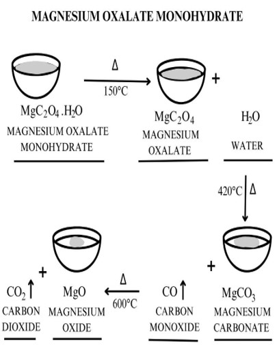

🔹 Step 1: Dehydration at 150°C
· A crucible containing magnesium oxalate monohydrate (MgC₂O₄·H₂O) is heated to 150°C.
· The reaction: MgC₂O₄·H₂O → MgC₂O₄ + H₂O
· Products: magnesium oxalate (solid remains in the crucible) and water (released as vapor).
🔹 Step 2: Partial Decomposition at 420°C
· Magnesium oxalate (MgC₂O₄) is further heated to 420°C.
· The reaction: MgC₂O₄ → MgCO₃ + CO (carbon monoxide)
· Products: magnesium carbonate (MgCO₃, solid) and carbon monoxide gas (CO, indicated by an upward arrow).
🔹 Step 3: Final Decomposition at 600°C
· Magnesium carbonate (MgCO₃) is heated to 600°C.
· The reaction: MgCO₃ → MgO + CO₂
· Products: magnesium oxide (MgO, solid) and carbon dioxide gas (CO₂, shown with an upward arrow).
Overall Purpose of the Diagram:
The image illustrates the stepwise thermal decomposition of magnesium oxalate monohydrate, showing how heat drives off water, produces carbon monoxide and carbon dioxide, and leaves behind solid magnesium oxide.
Activity 2.6:

A labeled diagram shows a crucible containing solid ammonium nitrate (NH₄NO₃). An arrow indicates heating to 300°C, leading to the decomposition reaction:
NH₄NO₃ (s) → 2H₂O (g) + N₂O (g). Water vapor and nitrous oxide gases are shown escaping upward.
Activity: 2.8
1. Ans: a
Ca(OH)2(s) →CaO (S) +H2O(g)
74.1g 56.1g 18g
% weight loss =  x 100 = 24.3%
Ans: b
6PbO(s) + O2(g) → 2Pb3O4(S)
1339.2 g 1371.2 g
% weight gain =  x 100 = 2.4%

TG for ‘b’ TG for ‘a’
2. Ans
The decrease in weight corresponds to the amount of carbon dioxide lost due to the decomposition of calcium carbonate present in the mixture as per the following reaction:
CaCO3(s)→ CaO (s) + CO2(g)↑
Weight loss = 250.6-190.8 = 59.8 mg
1mol of CaCO3 ≡ 1 mol of CO2
100.1mg of CaCO3≡ 44mg of CO2
? ≡ 59.8 mg of CO2
=  = 136.05 mg of CaCO3
Weight of the sample = 250.6 mg = mixture of CaCO3 &CaO
250.6 mg of mixture = 136.05 mg of CaCO3
100 mg of mixture = 
= 54.29% of CaCO3
3.Ans
CaC2O4.H2O(s)→ CaC2O4(s) + H2O ↑
CaC2O4(s) → CaCO3(s) + CO(g) ↑
CaCO3(s) →CaO(s) + CO2(g) ↑
ii. Calculate the % weight loss at each step.
% weight loss =  x 100
x 100
% weight loss at step 1 =  = 12.32
% weight loss at step 2 =  = 21.89
% weight loss at step 3 =  = 43.95
Activity 3:
The record shown is that of a DTA experiment since the ordinate plot ∆T which is a differential temperature. The downward direction of the peak indicates that a endothermic reaction has occurred. This in turn implies that the corresponding enthalpy change (∆H) must have been positive ie the value of enthalpy after the thermal effect was greater than its value before. This means that the sample took in heat during the reaction. Furthermore, there is evidence of a change in the heat capacity as the temperature is increased beyond the thermal transition. This is shown by the displacement of the baseline just beyond the end.
Answers: Select from the following list
[upward/downward, free energy/heat capacity, greater/less, DTG/DTA, base-line/background, derivative/differential, took in/gave out, negative/positive, enthalpy/entropy, before/after/during, exothermic/endothermic/isothermal, abscissa/ordinate, distortion/displacement.]
Activity 4.1: Read each of the statements and mark them as True or False
(i) In DSC the sample and reference positions are provided with their own separate heating sources, so that the assembly may be operated on a ‘null balance’ basis. T
(ii) In DTA the equipment is so designed that the temperature of the sample is equal to that of the reference material at every point in the heating programme. F
(iii) Chemical decompositions which give rise to weight changes may be detected by DTA and DSC. T
(iv) The main components of a conventional differential thermal analyser consist of following: F (programmer missing)
a) The sample/reference holder
b) The thermocouple
c) The furnace
d) The amplifier
e) The recorder
Activity 4.2:
If ∆H < 0, the system has undergone an endothermic/ exothermic change which means
Ts > TR [Choose the correct option: =, <, >]
Conversely ∆H > 0 means endothermic change and Ts < TR [Choose the correct option: =, <, >]
In order to keep ∆T = 0 [∆T = Ts – TR]
● In case of an endothermic reaction we must provide heat to sample/reference.
● In case of an exothermic reaction we must provide heat to sample/reference
Activity 4.3: Observe the DSC curve given in ‘figure 4.3a.’ and answer the following questions.
⮚ How many transitions are seen in the above diagram?
Ans: Two
⮚ Do you see any endotherm or exotherm? If yes, how many?
Ans: One endotherm and one exotherm.
⮚ What does the endo or exothermic nature of the transition tell you about transition or ∆H value?
Ans: Endotherm: + ve ∆H (heat is absorbed) Exotherm: -ve ∆H (heat is given out)
⮚ Is the DSC curve of PET useful in predicting stability of the polymer? Justify your answer.
Ans: Yes, the melting point of any polymer is an important characteristic. It is the minimum temperature for processing the polymer and maximum temperature for using it. In addition, the glass transition temperature is useful since beyond this there is change in some of the physical properties of the polymer.