13.4: Flow Injection Analysis

The focus of this chapter is on methods in which we measure a time-dependent signal. Chemical kinetic methods and radiochemical methods are two examples. In this section we consider the technique of flow injection analysis in which we inject the sample into a flowing carrier stream that gives rise to a transient signal at the detector. Because the shape of this transient signal depends on the physical and chemical kinetic processes that take place in the carrier stream during the time between injection and detection, we include flow injection analysis in this chapter.

Theory and Practice

Flow injection analysis (FIA) was developed in the mid-1970s as a highly efficient technique for the automated analyses of samples [see, for example, (a) Ruzicka, J.; Hansen, E. H. Anal. Chim. Acta 1975, 78, 145–157; (b) Stewart, K. K.; Beecher, G. R.; Hare, P. E. Anal. Biochem. 1976, 70, 167–173; (c) Valcárcel, M.; Luque de Castro, M. D. Flow Injection Analysis: Principles and Applications, Ellis Horwood: Chichester, England, 1987]. Unlike the centrifugal analyzer described earlier in this chapter (see Figure 13.2.8), in which the number of samples is limited by the transfer disk’s size, FIA allows for the rapid, sequential analysis of an unlimited number of samples. FIA is one example of a continuous-flow analyzer, in which we sequentially introduce samples at regular intervals into a liquid carrier stream that transports them to the detector.

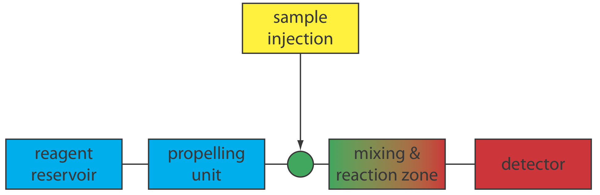
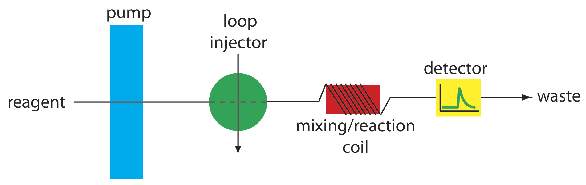
A schematic diagram detailing the basic components of a flow injection analyzer is shown in Figure 13.4.1 . The reagent that serves as the carrier is stored in a reservoir, and a propelling unit maintains a constant flow of the carrier through a system of tubing that comprises the transport system. We inject the sample directly into the flowing carrier stream, where it travels through one or more mixing and reaction zones before it reaches the detector’s flow-cell. Figure 13.4.1 is the simplest design for a flow injection analyzer, which consists of a single channel and a single reagent reservoir. Multiple channel instruments that merge together separate channels, each of which introduces a new reagent into the carrier stream, also are possible. A more detailed discussion of FIA instrumentation is found in the next section.

Figure 13.4.1 . Schematic diagram of a simple flow injection analyzer showing its basic components. After its injection into the carrier stream the samples mixes and reacts with the carrier stream’s reagents before reaching the detector.

When we first inject a sample into the carrier stream it has the rectangular flow profile of width w shown in Figure 13.4.2 a. As the sample moves through the mixing zone and the reaction zone, the width of its flow profile increases as the sample disperses into the carrier stream. Dispersion results from two processes: convection due to the flow of the carrier stream and diffusion due to the concentration gradient between the sample and the carrier stream. Convection occurs by laminar flow. The linear velocity of the sample at the tube’s walls is zero, but the sample at the center of the tube moves with a linear velocity twice that of the carrier stream. The result is the parabolic flow profile shown in Figure 13.4.2 b. Convection is the primary means of dispersion in the first 100 ms following the sample’s injection.

Figure 13.4.2 . Effect of dispersion on the shape of a sample’s flow profile, shown in blue, at different times during a flow injection analysis: (a) at injection; (b) when convection dominates dispersion; (c) when convection and diffusion contribute to dispersion; and (d) when diffusion dominates dispersion. The red line shows the width, w, of the samples flow profile.

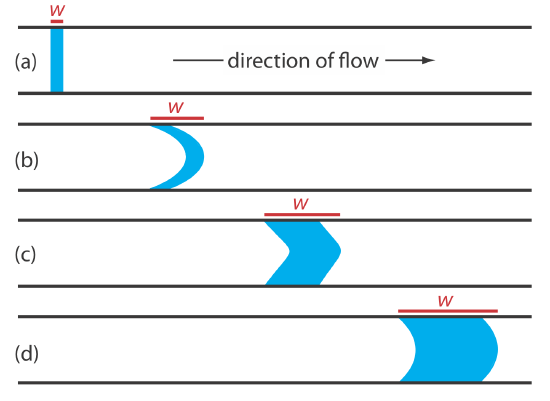
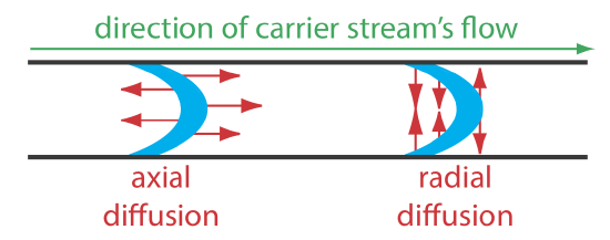
The second contribution to the sample’s dispersion is diffusion due to the concentration gradient that exists between the sample and the carrier stream. As shown in Figure 13.20, diffusion occurs parallel (axially) and perpendicular (radially) to the direction in which the carrier stream is moving. Only radial diffusion is important in a flow injection analysis. Radial diffusion decreases the sample’s linear velocity at the center of the tubing, while the sample at the edge of the tubing experiences an increase in its linear velocity. Diffusion helps to maintain the integrity of the sample’s flow profile (Figure 13.4.2 c) and prevents adjacent samples in the carrier stream from dispersing into one another. Both convection and diffusion make significant contributions to dispersion from approximately 3–20 s after the sample’s injection. This is the normal time scale for a flow injection analysis. After approximately 25 s, diffusion is the only significant contributor to dispersion, resulting in a flow profile similar to that shown in Figure 13.4.2 d.

Figure 13.4.3 . Illustration showing axial and radial diffusion. The blue band is the sample’s flow profile and the red arrows indicate the direction of diffusion.

An FIA curve, or fiagram, is a plot of the detector’s signal as a function of time. Figure 13.4.4 shows a typical fiagram for conditions in which both convection and diffusion contribute to the sample’s dispersion. Also shown on the figure are several parameters that characterize a sample’s fiagram. Two parameters define the time for a sample to move from the injector to the detector. Travel time, t_a, is the time between the sample’s injection and the arrival of its leading edge at the detector. Residence time, T, on the other hand, is the time required to obtain the maximum signal. The difference between the residence time and the travel time is \(t^{\prime}\), which approaches zero when convection is the primary means of dispersion, and increases in value as the contribution from diffusion becomes more important.

Figure 13.4.4 . Typical fiagram for flow injection analysis showing the detector's response as a function of time. See the text for an explanation of the parameters, \(t_a\), \(t^{\prime}\), \(\Delta t\), \(T^{\prime}\), and \(h\).

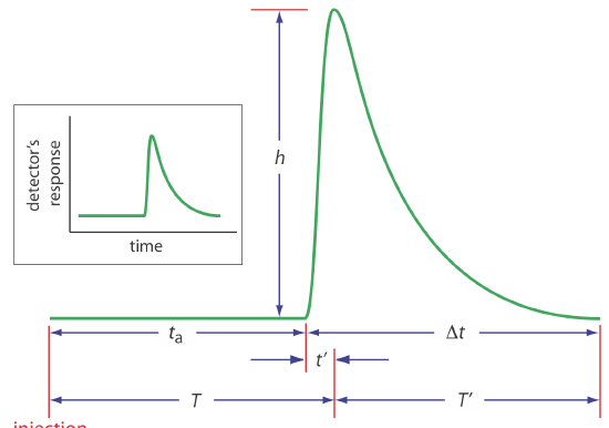
The time required for the sample to pass through the detector’s flow cell—and for the signal to return to the baseline—is also described by two parameters. The baseline-to-baseline time, \(\Delta t\), is the time between the arrival of the sample’s leading edge to the departure of its trailing edge. The elapsed time between the maximum signal and its return to the baseline is the return time, \(T^{\prime}\). The final characteristic parameter of a fiagram is the sample’s peak height, h.

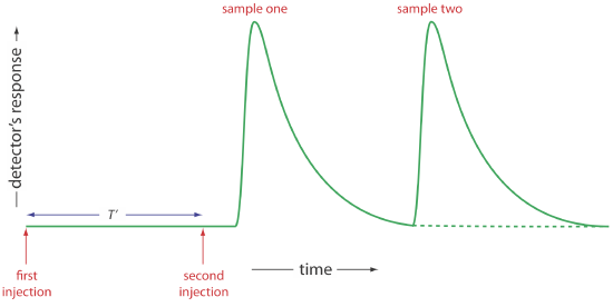
Of the six parameters shown in Figure 13.4.4 , the most important are peak height and the return time. Peak height is important because it is directly or indirectly related to the analyte’s concentration. The sensitivity of an FIA method, therefore, is determined by the peak height. The return time is important because it determines the frequency with which we may inject samples. Figure 13.4.5 shows that if we inject a second sample at a time \(T^{\prime}\) after we inject the first sample, there is little overlap of the two FIA curves. By injecting samples at intervals of \(T^{\prime}\), we obtain the maximum possible sampling rate.

Figure 13.4.5 . Effect of return time, \(T^{\prime}\), on sampling frequency.

Peak heights and return times are influenced by the dispersion of the sample’s flow profile and by the physical and chemical properties of the flow injection system. Physical parameters that affect h and \(T^{\prime}\) include the volume of sample we inject, the flow rate, the length, diameter and geometry of the mixing zone and the reaction zone, and the presence of junctions where separate channels merge together. The kinetics of any chemical reactions between the sample and the reagents in the carrier stream also influ-ence the peak height and return time.

Unfortunately, there is no good theory that we can use to consistently predict the peak height and the return time for a given set of physical and chemical parameters. The design of a flow injection analyzer for a particular analytical problem still occurs largely by a process of experimentation. Nevertheless, we can make some general observations about the effects of physical and chemical parameters. In the absence of chemical effects, we can improve sensitivity—that is, obtain larger peak heights—by injecting larger samples, by increasing the flow rate, by decreasing the length and diameter of the tubing in the mixing zone and the reaction zone, and by merging separate channels before the point where the sample is injected. With the exception of sample volume, we can increase the sampling rate—that is, decrease the return time—by using the same combination of physical parameters. Larger sample volumes, however, lead to longer return times and a decrease in sample throughput. The effect of chemical reactivity depends on whether the species we are monitoring is a reactant or a product. For example, if we are monitoring a reactant, we can improve sensitivity by choosing conditions that decrease the residence time, T, or by adjusting the carrier stream’s composition so that the reaction occurs more slowly.

Instrumentation

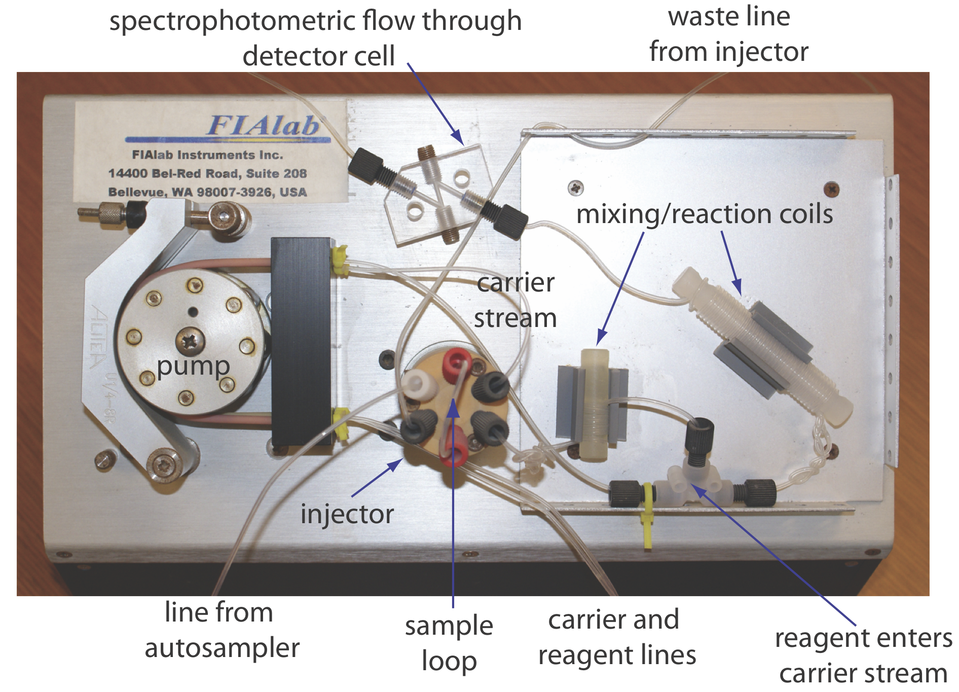
The basic components of a flow injection analyzer are shown in Figure 13.4.6 and include a pump to propel the carrier stream and the reagent streams, a means to inject the sample into the carrier stream, and a detector to monitor the composition of the carrier stream. Connecting these units is a transport system that brings together separate channels and provides time for the sample to mix with the carrier stream and to react with the reagent streams. We also can incorporate separation modules into the transport system. Each of these components is considered in greater detail in this section.

Figure 13.4.6 . Example of a typical flow injection analyzer that shows the pump, the injector, the transport system, which consists of mixing/reaction coils and junctions, and the detector (minus the spectrophotometer). This particular configuration has two channels: the carrier stream and a reagent line.

Propelling Unit

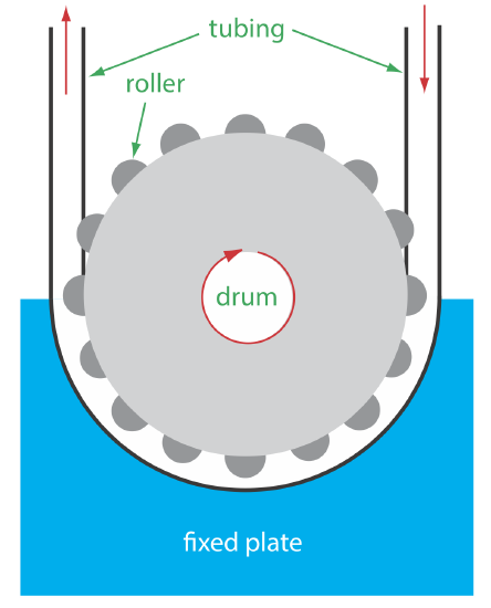
The propelling unit moves the carrier stream through the flow injection analyzer. Although several different propelling units have been used, the most common is a peristaltic pump, which, as shown in Figure 13.4.7 , consists of a set of rollers attached to the outside of a rotating drum. Tubing from the reagent reservoirs fits between the rollers and a fixed plate. As the drum rotates the rollers squeeze the tubing, forcing the contents of the tubing to move in the direction of the rotation. Peristaltic pumps provide a constant flow rate, which is controlled by the drum’s speed of rotation and the inner diameter of the tubing. Flow rates from 0.0005–40 mL/min are possible, which is more than adequate to meet the needs of FIA where flow rates of 0.5–2.5 mL/min are common. One limitation to a peristaltic pump is that it produces a pulsed flow—particularly at higher flow rates—that may lead to oscillations in the signal.

Figure 13.4.7 . Schematic diagram of a peristaltic pump.

Injector

The sample, typically 5–200 μL, is injected into the carrier stream. Although syringe injections through a rubber septum are possible, the more common method—as seen in Figure 13.4.6 —is to use a rotary, or loop injector similar to that used in an HPLC. This type of injector provides for a reproducible sample volume and is easily adaptable to automation, an important feature when high sampling rates are needed.

Detector

The most common detectors for flow injection analysis are the electrochemical and optical detectors used in HPLC. These detectors are discussed in Chapter 12 and are not considered further in this section. FIA detectors also have been designed around the use of ion selective electrodes and atomic absorption spectroscopy.

Transport System

The heart of a flow injection analyzer is the transport system that brings together the carrier stream, the sample, and any reagents that react with the sample. Each reagent stream is considered a separate channel, and all channels must merge before the carrier stream reaches the detector. The complete transport system is called a manifold.

The simplest manifold has a single channel, the basic outline of which is shown in Figure 13.4.8 . This type of manifold is used for direct analysis of analyte that does not require a chemical reaction. In this case the carrier stream serves only as a means for rapidly and reproducibly transporting the sample to the detector. For example, this manifold design has been used for sample introduction in atomic absorption spectroscopy, achieving sampling rates as high as 700 samples/h. A single-channel manifold also is used for determining a sample’s pH or determining the concentration of metal ions using an ion selective electrode.

Figure 13.4.8 . Example of a single-channel manifold in which the reagent serves as the carrier stream and as a species that reacts with the sample. The mixing/reaction coil is wrapped around a plastic cylinder.

We can also use the single-channel manifold in Figure 13.4.8 for an analysis in which we monitor the product of a chemical reaction between the sample and a reactant. In this case the carrier stream both transports the sample to the detector and reacts with the sample. Because the sample must mix with the carrier stream, a lower flow rate is used. One example is the determination of chloride in water, which is based on the following sequence of reactions.

\[\mathrm{Hg}(\mathrm{SCN})_{2}(a q)+2 \mathrm{Cl}^{-}(a q) \rightleftharpoons \: \mathrm{HgCl}_{2}(a q)+2 \mathrm{SCN}^{-}(a q) \nonumber\]

\[\mathrm{Fe}^{3+}(a q)+\mathrm{SCN}^{-}(a q) \rightleftharpoons \mathrm{Fe}(\mathrm{SCN})^{2+}(a q) \nonumber\]

The carrier stream consists of an acidic solution of Hg(SCN)₂ and Fe³⁺. Injecting a sample that contains chloride into the carrier stream displaces thiocyanate from Hg(SCN)₂. The displaced thiocyanate then reacts with Fe³⁺ to form the red-colored Fe(SCN)²⁺ complex, the absorbance of which is monitored at a wavelength of 480 nm. Sampling rates of approximately 120 samples per hour have been achieved with this system [Hansen, E. H.; Ruzicka, J. J. Chem. Educ. 1979, 56, 677–680].

Most flow injection analyses that include a chemical reaction use a manifold with two or more channels. Including additional channels provides more control over the mixing of reagents and the interaction between the reagents and the sample. Two configurations are possible for a dual-channel system. A dual-channel manifold, such as the one shown in Figure 13.4.9 a, is used when the reagents cannot be premixed because of their reactivity. For example, in acidic solutions phosphate reacts with molybdate to form the heteropoly acid H₃P(Mo₁₂O₄₀). In the presence of ascorbic acid the molybdenum in the heteropoly acid is reduced from Mo(VI) to Mo(V), forming a blue-colored complex that is monitored spectrophotometrically at 660 nm [Hansen, E. H.; Ruzicka, J. J. Chem. Educ. 1979, 56, 677–680]. Because ascorbic acid reduces molybdate, the two reagents are placed in separate channels that merge just before the loop injector.

Figure 13.4.9 . Two examples of a dual-channel manifold for flow injection analysis. In (a) the two channels merge before the loop injector, and in (b) the two channels merge after the loop injector.

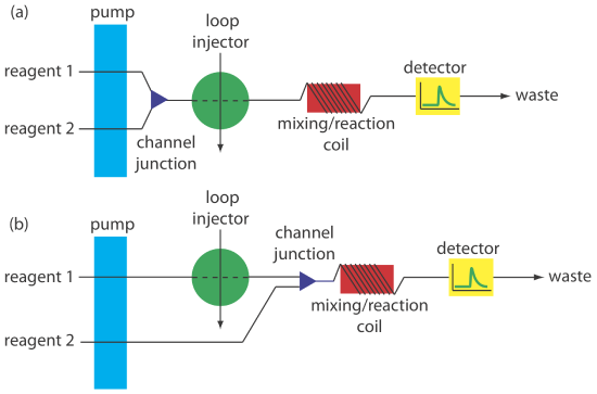
A dual-channel manifold also is used to add a second reagent after injecting the sample into a carrier stream, as shown in Figure 13.4.9 b. This style of manifold is used for the quantitative analysis of many analytes, including the determination of a wastewater’s chemical oxygen demand (COD) [Korenaga, T.; Ikatsu, H. Anal. Chim. Acta 1982, 141, 301–309]. Chemical oxygen demand is a measure of the amount organic matter in the wastewater sample. In the conventional method of analysis, COD is determined by refluxing the sample for 2 h in the presence of acid and a strong oxidizing agent, such as K₂Cr₂O₇ or KMnO₄. When refluxing is complete, the amount of oxidant consumed in the reaction is determined by a redox titration. In the flow injection version of this analysis, the sample is injected into a carrier stream of aqueous H₂SO₄, which merges with a solution of the oxidant from a secondary channel. The oxidation reaction is kinetically slow and, as a result, the mixing coil and the reaction coil are very long—typically 40 m—and submerged in a thermostated bath. The sampling rate is lower than that for most flow injection analyses, but at 10–30 samples/h it is substantially greater than the redox titrimetric method.

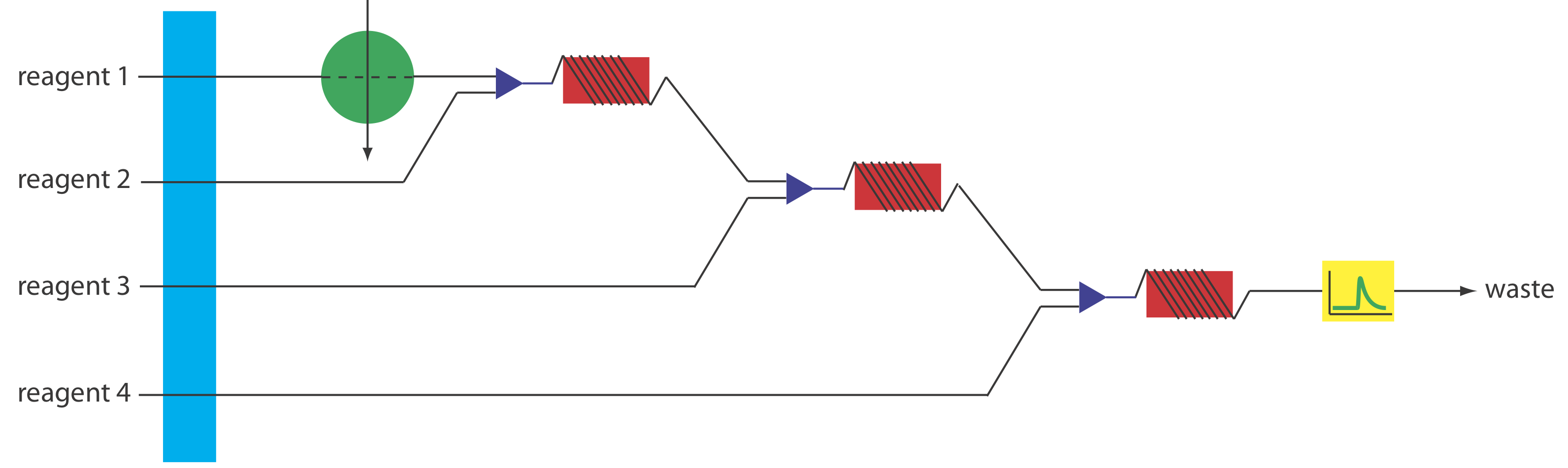
More complex manifolds involving three or more channels are common, but the possible combination of designs is too numerous to discuss. One example of a four-channel manifold is shown in Figure 13.4.10 .

Figure 13.4.10 . Example of a four-channel manifold for a flow injection analysis.

Separation Modules

By incorporating a separation module into the flow injection manifold we can include a separation—dialysis, gaseous diffusion and liquid-liquid extractions are examples—in a flow injection analysis. Although these separations are never complete, they are reproducible if we carefully control the experimental conditions.

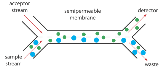
Dialysis and gaseous diffusion are accomplished by placing a semipermeable membrane between the carrier stream containing the sample and an acceptor stream, as shown in Figure 13.4.11 . As the sample stream passes through the separation module, a portion of those species that can cross the semipermeable membrane do so, entering the acceptor stream. This type of separation module is common for the analysis of clinical samples, such as serum and urine, where a dialysis membrane separates the analyte from its complex matrix. Semipermeable gaseous diffusion membranes are used for the determination of ammonia and carbon dioxide in blood. For example, ammonia is determined by injecting the sample into a carrier stream of aqueous NaOH. Ammonia diffuses across the semipermeable membrane into an acceptor stream that contains an acid–base indicator. The resulting acid–base reaction between ammonia and the indicator is monitored spectrophotometrically.

Figure 13.4.11 . Separation module for a flow injection analysis using a semipermeable membrane. The smaller green solutes can pass through the semipermeable membrane and enter the acceptor stream, but the larger blue solutes cannot. Although the separation is not complete—note that some of the green solute remains in the sample stream and exits as waste—it is reproducible if we do not change the experimental conditions.

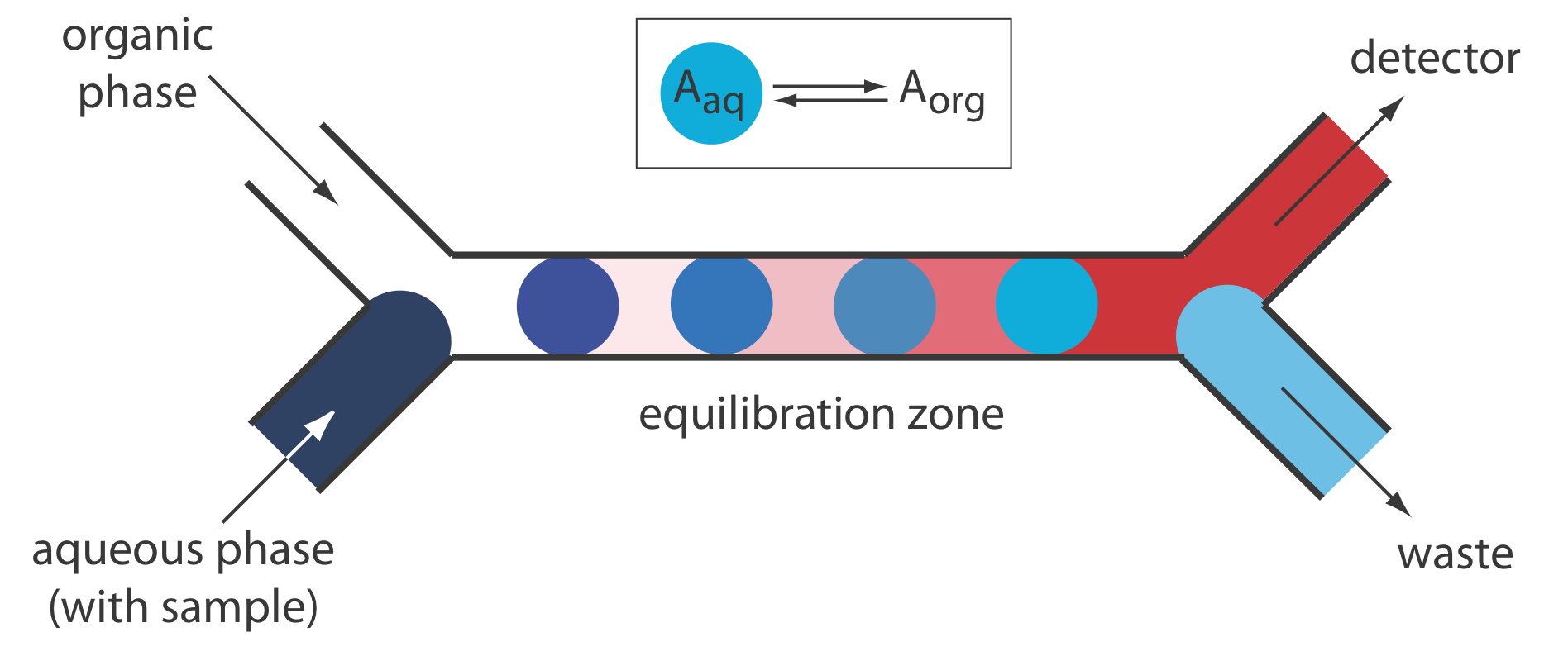
Liquid–liquid extractions are accomplished by merging together two immiscible fluids, each carried in a separate channel. The result is a segmented flow through the separation module, consisting of alternating portions of the two phases. At the outlet of the separation module the two fluids are separated by taking advantage of the difference in their densities. Figure 13.4.12 shows a typical configuration for a separation module in which the sample is injected into an aqueous phase and extracted into a less dense organic phase that passes through the detector.

Figure 13.4.12 . Separation module for flow injection analysis using a liquid–liquid extraction. The inset shows the equilibrium reaction. As the sample moves through the equilibration zone, the analyte extracts into the organic phase.

Quantitative Applications

In a quantitative flow injection method a calibration curve is determined by injecting a series of external standards that contain known concentrations of analyte. The calibration curve’s format—examples include plots of absorbance versus concentration and of potential versus concentration—depends on the method of detection. Calibration curves for standard spectroscopic and electrochemical methods are discussed in Chapter 10 and in Chapter 11, respectively and are not considered further in this chapter.

Flow injection analysis has been used to analyze a wide variety of samples, including environmental, clinical, agricultural, industrial, and pharmaceutical samples. The majority of analyses involve environmental and clinical samples, which is the focus of this section.

Quantitative flow injection methods have been developed for cationic, anionic, and molecular pollutants in wastewater, freshwaters, groundwaters, and marine waters, three examples of which were described in the previous section. Table 13.4.1 provides a partial listing of other analytes that have been determined using FIA, many of which are modifications of standard spectrophotometric and potentiometric methods. An additional advantage of FIA for environmental analysis is the ability to provide for the continuous, in situ monitoring of pollutants in the field [Andrew, K. N.; Blundell, N. J.; Price, D.; Worsfold, P. J. Anal. Chem. 1994, 66, 916A–922A].

Table 13.4.1 . Selected Flow Injection Analysis Methods for Environmental Samples

analyte	sample	sample volume (µL)	concentration range	sampling frequency (h^–1)
Ca^2^+	freshwater	20	0.8–7.2 ppm	80
Cu^2^+	groundwater	70–700	100–400 ppb	20
Pb^2+	groundwater	70–700	0–40 ppb	20
Zn^2^+	seawater	1000	1–100 ppb	30–60
\(\text{NH}_4^+\)	seawater	60	0.18–18.1 ppb	288
\(\text{NO}_3^-\)	rainwater	1000	1–10 ppb	40
\(\text{SO}_4^{2-}\)	freshwater	400	4–140 ppb	180
CN^–	industrial	10	0.3–100 ppm	40
Source: Adapted from Valcárcel, M.; Luque de Castro, M. D. Flow-Injection Analysis: Principles and Practice, Ellis Horwood: Chichester, England, 1987.

As noted in Chapter 9, several standard methods for the analysis of water involve an acid–base, complexation, or redox titration. It is easy to adapt these titrations to FIA using a single-channel manifold similar to that shown in Figure 13.4.8 [Ramsing, A. U.; Ruzicka, J.; Hansen, E. H. Anal. Chim. Acta 1981, 129, 1–17]. The titrant—whose concentration must be stoichiometrically less than that of the analyte—and a visual indicator are placed in the reagent reservoir and pumped continuously through the manifold. When we inject the sample it mixes thoroughly with the titrant in the carrier stream. The reaction between the analyte, which is in excess, and the titrant produces a relatively broad rectangular flow profile for the sample. As the sample moves toward the detector, additional mixing oc- curs and the width of the sample’s flow profile decreases. When the sample passes through the detector, we determine the width of its flow profile, \(\Delta T\), by monitoring the indicator’s absorbance. A calibration curve of \(\Delta T\) versus log[analyte] is prepared using standard solutions of analyte.

Flow injection analysis has also found numerous applications in the analysis of clinical samples, using both enzymatic and nonenzymatic methods. Table 13.4.2 summarizes several examples.

Table 13.4.2 . Selected Flow Injection Analysis Methods for Clinical Samples

analyte	sample	sample volume (µL)	concentration range	sampling frequency (h^–1)
nonenzymatic methods
Cu^2+	serum	20	0.7–1.5 ppm	70
Cl^–	serum	60	50–150 meq/L	125
\(\text{PO}_4^{3-}\)	serum	200	10–60 ppm	130
total CO2	serum	50	10–50 mM	70
chlorpromazine	blood plasma	200	1.5–9 \(\mu \text{M}\)	24
enzymatic methods
glucose	blood serum	26.5	0.5–15 mM	60
urea	blood serum	30	4–20 mM	60
ethanol	blood	30	5–30 ppm	50
Source: Adapted from Valcárcel, M.; Luque de Castro, M. D. Flow-Injection Analysis: Principles and Practice, Ellis Horwood: Chichester, England, 1987.

The best way to appreciate the theoretical and the practical details discussed in this section is to carefully examine a typical analytical method. Although each method is unique, the following description of the determination of phosphate provides an instructive example of a typical procedure. The description here is based on Guy, R. D.; Ramaley, L.; Wentzell, P. D. “An Experiment in the Sampling of Solids for Chemical Analysis,” J. Chem. Educ. 1998, 75, 1028–1033. As the title suggests, the primary focus of this chapter is on sampling. A flow injection analysis, however, is used to analyze samples.

Representative Method 13.4.1: Determination of Phosphate by FIA

Description of Method

The FIA determination of phosphate is an adaptation of a standard spectrophotometric analysis for phosphate. In the presence of acid, phosphate reacts with ammonium molybdate to form a yellow-colored complex in which molybdenum is present as Mo(VI).

\[\mathrm{H}_{3} \mathrm{PO}_{4}(a q)+12 \mathrm{H}_{2} \mathrm{MoO}_{4}(a q) \leftrightharpoons \: \mathrm{H}_{3} \mathrm{P}\left(\mathrm{Mo}_{12} \mathrm{O}_{40}\right)(a q)+12 \mathrm{H}_{2} \mathrm{O}(\mathrm{l}) \nonumber\]

In the presence of a reducing agent, such as ascorbic acid, the yellow-colored complex is reduced to a blue-colored complex of Mo(V).

Procedure

Prepare the following three solutions: (a) 5.0 mM ammonium molybdate in 0.40 M HNO₃; (b) 0.7% w/v ascorbic acid in 1% v/v glycerin; and a (c) 100.0 ppm phosphate standard using KH₂PO₄. Using the phosphate standard, prepare a set of external standards with phosphate concentrations of 10, 20, 30, 40, 50 and 60 ppm. Use a manifold similar to that shown in Figure 13.4.9 a, placing a 50-cm mixing coil between the pump and the loop injector and a 50-cm reaction coil between the loop injector and the detector. For both coils, use PTFE tubing with an internal diameter of 0.8 mm. Set the flow rate to 0.5 mL/min. Prepare a calibration curve by injecting 50 μL of each standard, measuring the absorbance at 650 nm. Samples are analyzed in the same manner.

Questions

1. How long does it take a sample to move from the loop injector to the detector?

The reaction coil is 50-cm long with an internal diameter of 0.8 mm. The volume of this tubing is

\[V=l \pi r^{2}=50 \mathrm{cm} \times 3.14 \times\left(\frac{0.08 \mathrm{cm}}{2}\right)^{2}=0.25 \mathrm{cm}^{3}=0.25 \mathrm{mL} \nonumber\]

With a flow rate of 0.5 mL/min, it takes about 30 s for a sample to pass through the system.

2. The instructions for the standard spectrophotometric method indicate that the absorbance is measured 5–10 min after adding the ascorbic acid. Why is this waiting period necessary in the spectrophotometric method, but not necessary in the FIA method?

The reduction of the yellow-colored Mo(VI) complex to the blue-colored Mo(V) complex is a slow reaction. In the standard spectro-photometric method it is difficult to control reproducibly the time between adding the reagents to the sample and measuring the sample’s absorbance. To achieve good precision we allow the reaction to proceed to completion before we measure the absorbance. As seen by the answer to the previous question, in the FIA method the flow rate and the dimensions of the reaction coil determine the reaction time. Because this time is controlled precisely, the reaction occurs to the same extent for all standards and samples. A shorter reaction time has the advantage of allowing for a higher throughput of samples.

3. The spectrophotometric method recommends using phosphate standards of 2–10 ppm. Explain why the FIA method uses a different range of standards.

In the FIA method we measure the absorbance before the formation of the blue-colored Mo(V) complex is complete. Because the absorbance for any standard solution of phosphate is always smaller when using the FIA method, the FIA method is less sensitive and higher concentrations of phosphate are necessary.

4. How would you incorporate a reagent blank into the FIA analysis?

A reagent blank is obtained by injecting a sample of distilled water in place of the external standard or the sample. The reagent blank’s absorbance is subtracted from the absorbances obtained for the standards and samples.

Example 13.4.1

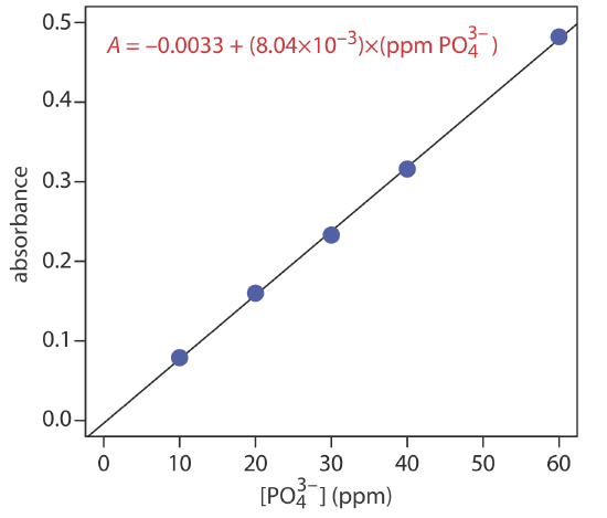
The following data were obtained for a set of external standards when using Representative Method 13.4.1 to analyze phosphate in a wastewater sample.

[\(\text{PO}_4^{3-}\)] (ppm)	absorbance
10.00	0.079
20.00	0.160
30.00	0.233
40.00	0.316
60.00	0.482

What is the concentration of phosphate in a sample if it gives an absorbance of 0.287?

Solution

Figure 13.4.13 shows the external standards calibration curve and the calibration equation. Substituting in the sample’s absorbance gives the con- centration of phosphate in the sample as 36.1 ppm.

Figure 13.4.13 . Calibration curve and equation for the data in Example 13.4.1 .

Evaluation

The majority of flow injection analysis applications are modifications of conventional titrimetric, spectrophotometric, and electrochemical methods of analysis; thus, it is appropriate to compare FIA methods to these conventional methods. The scale of operations for FIA allows for the routine analysis of minor and trace analytes, and for macro, meso, and micro samples. The ability to work with microliter injection volumes is useful when the sample is scarce. Conventional methods of analysis usually have smaller detection limits.

The accuracy and precision of FIA methods are comparable to conven- tional methods of analysis; however, the precision of FIA is influenced by several variables that do not affect conventional methods, including the stability of the flow rate and the reproducibility of the sample’s injection. In addition, results from FIA are more susceptible to temperature variations.

In general, the sensitivity of FIA is less than that for conventional methods of analysis for at least two reasons. First, as with chemical kinetic methods, measurements in FIA are made under nonequilibrium conditions when the signal has yet to reach its maximum value. Second, dispersion dilutes the sample as it moves through the manifold. Because the variables that affect sensitivity are known, we can design the FIA manifold to optimize the method’s sensitivity.

Selectivity for an FIA method often is better than that for the corresponding conventional method of analysis. In many cases this is due to the kinetic nature of the measurement process, in which potential interferents may react more slowly than the analyte. Contamination from external sources also is less of a problem because reagents are stored in closed reservoirs and are pumped through a system of transport tubing that is closed to the environment.

Finally, FIA is an attractive technique when considering time, cost, and equipment. When using an autosampler, a flow injection method can achieve very high sampling rates. A sampling rate of 20–120 samples/h is not unusual and sampling rates as high as 1700 samples/h are possible. Because the volume of the flow injection manifold is small, typically less than 2 mL, the consumption of reagents is substantially smaller than that for a conventional method. This can lead to a significant decrease in the cost per analysis. Flow injection analysis does require the need for additional equipment—a pump, a loop injector, and a manifold—which adds to the cost of an analysis.

For a review of the importance of flow injection analysis, see Hansen, E. H.; Miró, M. “How Flow-Injection Analysis (FIA) Over the Past 25 Years has Changed Our Way of Performing Chemical Analyses,” TRAC, Trends Anal. Chem. 2007, 26, 18–26.