12.3: Optimizing Chromatographic Separations

Now that we have defined the solute retention factor, selectivity, and column efficiency we are able to consider how they affect the resolution of two closely eluting peaks. Because the two peaks have similar retention times, it is reasonable to assume that their peak widths are nearly identical. If the number of theoretical plates is the same for all solutes—not strictly true, but not a bad assumption—then from equation 12.2.15, the ratio t_r/w is a constant. If two solutes have similar retention times, then their peak widths must be similar. Equation 12.2.1, therefore, becomes

\[R_{A B}=\frac{t_{r, B}-t_{r, A}}{0.5\left(w_{B}+w_{A}\right)} \approx \frac{t_{r, B}-t_{r, A}}{0.5\left(2 w_{B}\right)}=\frac{t_{r, B}-t_{r, A}}{w_{B}} \label{12.1}\]

where B is the later eluting of the two solutes. Solving equation 12.2.15 for w_B and substituting into Equation \ref{12.1} leaves us with the following result.

\[R_{A B}=\frac{\sqrt{N_{B}}}{4} \times \frac{t_{r, B}-t_{r, A}}{t_{r, B}} \label{12.2}\]

Rearranging equation 12.2.8 provides us with the following equations for the retention times of solutes A and B.

\[t_{r, A}=k_{A} t_{\mathrm{m}}+t_{\mathrm{m}} \quad \text { and } \quad t_{\mathrm{r}, B}=k_{B} t_{\mathrm{m}}+t_{\mathrm{m}} \nonumber\]

After substituting these equations into Equation \ref{12.2} and simplifying, we have

\[R_{A B}=\frac{\sqrt{N_{B}}}{4} \times \frac{k_{B}-k_{A}}{1+k_{B}} \nonumber\]

Finally, we can eliminate solute A’s retention factor by substituting in equation 12.2.9. After rearranging, we end up with the following equation for the resolution between the chromatographic peaks for solutes A and B.

\[R_{A B}=\frac{\sqrt{N_{B}}}{4} \times \frac{\alpha-1}{\alpha} \times \frac{k_{B}}{1+k_{B}} \label{12.3}\]

In addition to resolution, another important factor in chromatography is the amount of time needed to elute a pair of solutes, which we can approximate using the retention time for solute B.

\[t_{r, s}=\frac{16 R_{AB}^{2} H}{u} \times\left(\frac{\alpha}{\alpha-1}\right)^{2} \times \frac{\left(1+k_{B}\right)^{3}}{k_{B}^{2}} \label{12.4}\]

where u is the mobile phase’s velocity.

Although Equation \ref{12.3} is useful for considering how a change in N, \(\alpha\), or k qualitatively affects resolution—which suits our purpose here—it is less useful for making accurate quantitative predictions of resolution, particularly for smaller values of N and for larger values of R. For more accurate predictions use the equation

\[R_{A B}=\frac{\sqrt{N}}{4} \times(\alpha-1) \times \frac{k_{B}}{1+k_{\mathrm{avg}}} \nonumber\]

where k_avg is (k_A + k_B)/2. For a derivation of this equation and for a deeper discussion of resolution in column chromatography, see Foley, J. P. “Resolution Equations for Column Chromatography,” Analyst, 1991, 116, 1275-1279.

Equation \ref{12.3} and Equation \ref{12.4} contain terms that correspond to column efficiency, selectivity, and the solute retention factor. We can vary these terms, more or less independently, to improve resolution and analysis time. The first term, which is a function of the number of theoretical plates (for Equation \ref{12.3}) or the height of a theoretical plate (for Equation \ref{12.4}), accounts for the effect of column efficiency. The second term is a function of \(\alpha\) and accounts for the influence of column selectivity. Finally, the third term in both equations is a function of k_B and accounts for the effect of solute B’s retention factor. A discussion of how we can use these parameters to improve resolution is the subject of the remainder of this section.

Using the Retention Factor to Optimize Resolution

One of the simplest ways to improve resolution is to adjust the retention factor for solute B. If all other terms in Equation \ref{12.3} remain constant, an increase in k_B will improve resolution. As shown by the green curve in Figure 12.3.1 , however, the improvement is greatest if the initial value of k_B is small. Once k_B exceeds a value of approximately 10, a further increase produces only a marginal improvement in resolution. For example, if the original value of k_B is 1, increasing its value to 10 gives an 82% improvement in resolution; a further increase to 15 provides a net improvement in resolution of only 87.5%.

Figure 12.3.1 . Effect of k_B on the resolution for a pair of solutes, R_AB, and the retention time for the later eluting solute, t_r,B. The y-axes display the resolution and retention time relative to their respective values when k_B is 1.00.

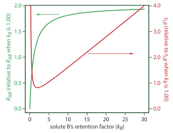
Any improvement in resolution from increasing the value of k_B generally comes at the cost of a longer analysis time. The red curve in Figure 12.3.1 shows the relative change in the retention time for solute B as a function of its retention factor. Note that the minimum retention time is for k_B = 2. Increasing k_B from 2 to 10, for example, approximately doubles solute B’s retention time.

The relationship between retention factor and analysis time in Figure 12.3.1 works to our advantage if a separation produces an acceptable resolution with a large k_B. In this case we may be able to decrease k_B with little loss in resolution and with a significantly shorter analysis time.

To increase k_B without changing selectivity, \(\alpha\), any change to the chromatographic conditions must result in a general, nonselective increase in the retention factor for both solutes. In gas chromatography, we can accomplish this by decreasing the column’s temperature. Because a solute’s vapor pressure is smaller at lower temperatures, it spends more time in the stationary phase and takes longer to elute. In liquid chromatography, the easiest way to increase a solute’s retention factor is to use a mobile phase that is a weaker solvent. When the mobile phase has a lower solvent strength, solutes spend proportionally more time in the stationary phase and take longer to elute.

Adjusting the retention factor to improve the resolution between one pair of solutes may lead to unacceptably long retention times for other solutes. For example, suppose we need to analyze a four-component mixture with baseline resolution and with a run-time of less than 20 min. Our initial choice of conditions gives the chromatogram in Figure 12.3.2 a. Although we successfully separate components 3 and 4 within 15 min, we fail to separate components 1 and 2. Adjusting conditions to improve the resolution for the first two components by increasing k₂ provides a good separation of all four components, but the run-time is too long (Figure 12.3.2 b). This problem of finding a single set of acceptable operating conditions is known as the general elution problem.

Figure 12.3.2 . Example showing the general elution problem in chromatography. See text for details.

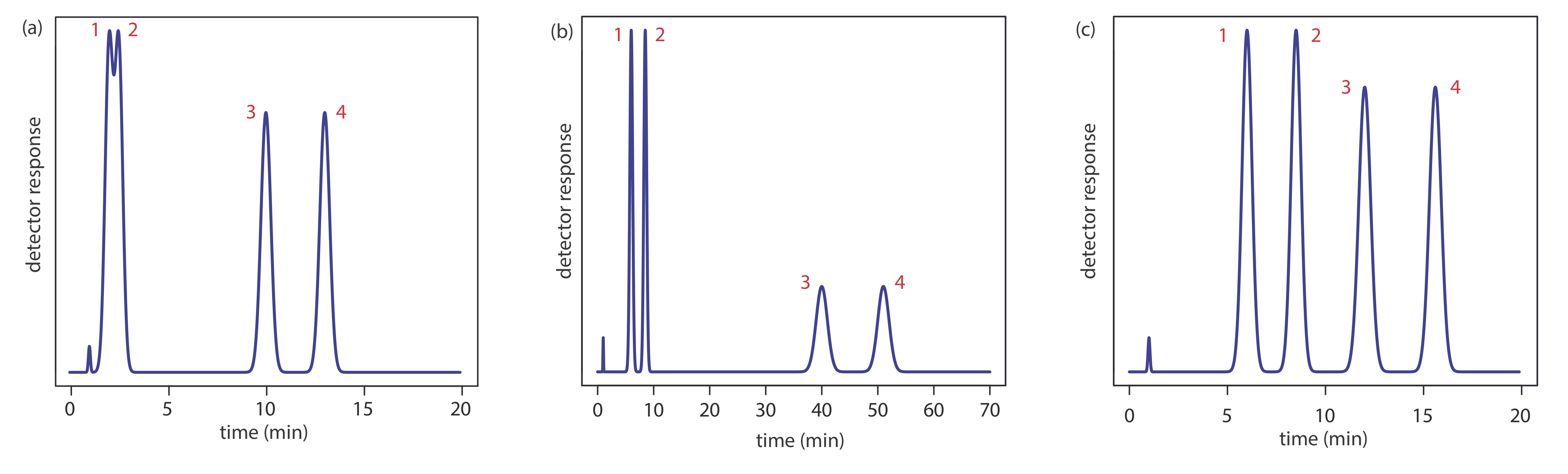
One solution to the general elution problem is to make incremental adjustments to the retention factor as the separation takes place. At the beginning of the separation we set the initial chromatographic conditions to optimize the resolution for early eluting solutes. As the separation progresses, we adjust the chromatographic conditions to decrease the retention factor—and, therefore, to decrease the retention time—for each of the later eluting solutes (Figure 12.3.2 c). In gas chromatography this is accomplished by temperature programming. The column’s initial temperature is selected such that the first solutes to elute are resolved fully. The temperature is then increased, either continuously or in steps, to bring off later eluting components with both an acceptable resolution and a reasonable analysis time. In liquid chromatography the same effect is obtained by increasing the solvent’s eluting strength. This is known as a gradient elution. We will have more to say about each of these in later sections of this chapter.

Using Selectivity to Optimize Resolution

A second approach to improving resolution is to adjust the selectivity, \(\alpha\). In fact, for \(\alpha \approx 1\) usually it is not possible to improve resolution by adjusting the solute retention factor, k_B, or the column efficiency, N. A change in \(\alpha\) often has a more dramatic effect on resolution than a change in k_B. For example, changing \(\alpha\) from 1.1 to 1.5, while holding constant all other terms, improves resolution by 267%. In gas chromatography, we adjust \(\alpha\) by changing the stationary phase; in liquid chromatography, we change the composition of the mobile phase to adjust \(\alpha\).

To change \(\alpha\) we need to selectively adjust individual solute retention factors. Figure 12.3.3 shows one possible approach for the liquid chromatographic separation of a mixture of substituted benzoic acids. Because the retention time of a compound’s weak acid form and its weak base form are different, its retention time will vary with the pH of the mobile phase, as shown in Figure 12.3.3 a. The intersections of the curves in Figure 12.3.3 a show pH values where two solutes co-elute. For example, at a pH of 3.8 terephthalic acid and p-hydroxybenzoic acid elute as a single chromatographic peak.

Figure 12.3.3 . Example showing how the mobile phase pH in liquid chromatography affects selectivity: (a) retention times for four substituted benzoic acids as a function of the mobile phase’s pH; (b) alpha values for three pairs of solutes that are difficult to separate. See text for details. The mobile phase is an acetic acid/sodium acetate buffer and the stationary phase is a nonpolar hydrocarbon. Data from Harvey, D. T.; Byerly, S.; Bowman, A.; Tomlin, J. “Optimization of HPLC and GC Separations Using Response Surfaces,” J. Chem. Educ. 1991, 68, 162–168.

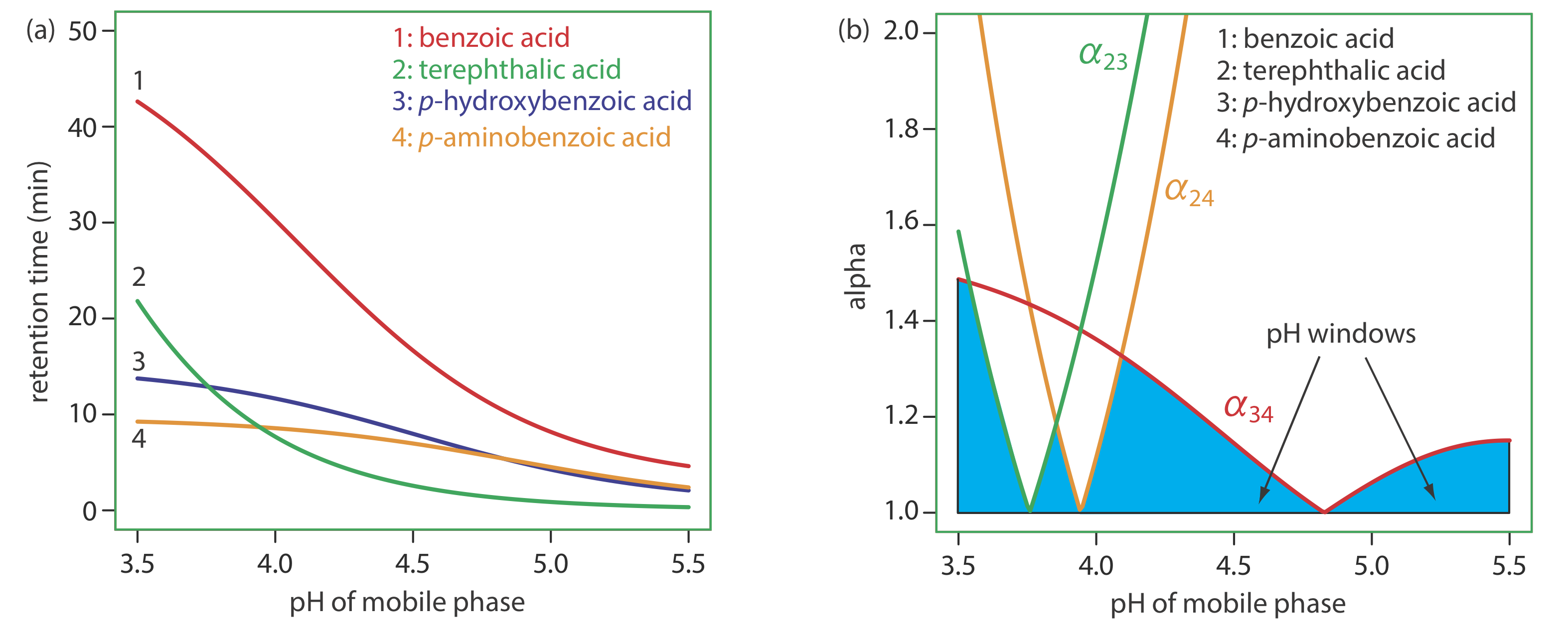
Figure 12.3.3 a shows that there are many pH values where some separation is possible. To find the optimum separation, we plot a for each pair of solutes. The red, green, and orange curves in Figure 12.3.3 b show the variation in a with pH for the three pairs of solutes that are hardest to separate (for all other pairs of solutes, \(\alpha\) > 2 at all pH levels). The blue shading shows windows of pH values in which at least a partial separation is possible—this figure is sometimes called a window diagram—and the highest point in each window gives the optimum pH within that range. The best overall separation is the highest point in any window, which, for this example, is a pH of 3.5. Because the analysis time at this pH is more than 40 min (Figure 12.3.3 a), choosing a pH between 4.1–4.4 might produce an acceptable separation with a much shorter analysis time.

Let’s use benzoic acid, C₆H₅COOH, to explain why pH can affect a solute’s retention time. The separation uses an aqueous mobile phase and a nonpolar stationary phase. At lower pHs, benzoic acid predominately is in its weak acid form, C₆H₅COOH, and partitions easily into the nonpolar stationary phase. At more basic pHs, however, benzoic acid is in its weak base form, C₆H₅COO^–. Because it now carries a charge, its solubility in the mobile phase increases and its solubility in the nonpolar stationary phase decreases. As a result, it spends more time in the mobile phase and has a shorter retention time.

Although the usual way to adjust pH is to change the concentration of buffering agents, it also is possible to adjust pH by changing the column’s temperature because a solute’s pK_a value is pH-dependent; for a review, see Gagliardi, L. G.; Tascon, M.; Castells, C. B. “Effect of Temperature on Acid–Base Equilibria in Separation Techniques: A Review,” Anal. Chim. Acta, 2015, 889, 35–57.

Using Column Efficiency to Optimize Resolution

A third approach to improving resolution is to adjust the column’s efficiency by increasing the number of theoretical plates, N. If we have values for k_B and \(\alpha\), then we can use Equation \ref{12.3} to calculate the number of theoretical plates for any resolution. Table 12.3.1 provides some representative values. For example, if \(\alpha\) = 1.05 and k_B = 2.0, a resolution of 1.25 requires approximately 24 800 theoretical plates. If our column provides only 12 400 plates, half of what is needed, then a separation is not possible. How can we double the number of theoretical plates? The easiest way is to double the length of the column, although this also doubles the analysis time. A better approach is to cut the height of a theoretical plate, H, in half, providing the desired resolution without changing the analysis time. Even better, if we can decrease H by more than 50%, it may be possible to achieve the desired resolution with an even shorter analysis time by also decreasing k_B or \(\alpha\).

Table 12.3.1 . Minimum Number of Theoretical Plates to Achieve Desired Resolution for Selected Values of k_B and \(\alpha\)

	RAB = 1.00		RAB = 1.25		RAB = 1.50
kB	\(\alpha = 1.05\)	\(\alpha = 1.10\)	\(\alpha = 1.05\)	\(\alpha = 1.10\)	\(\alpha = 1.05\)	\(\alpha = 1.10\)
0.5	63500	17400	99200	27200	143000	39200
1.0	28200	7740	44100	12100	63500	17400
1.5	19600	5380	30600	8400	44100	12100
2.0	15900	4360	24800	6810	35700	9800
3.0	12500	3440	19600	5380	28200	7740
5.0	10200	2790	15900	4360	22900	6270
10.0	8540	2340	13300	3660	19200	5270

To decrease the height of a theoretical plate we need to understand the experimental factors that affect band broadening. There are several theoretical treatments of band broadening. We will consider one approach that considers four contributions: variations in path lengths, longitudinal diffusion, mass transfer in the stationary phase, and mass transfer in the mobile phase.

Multiple Paths: Variations in Path Length

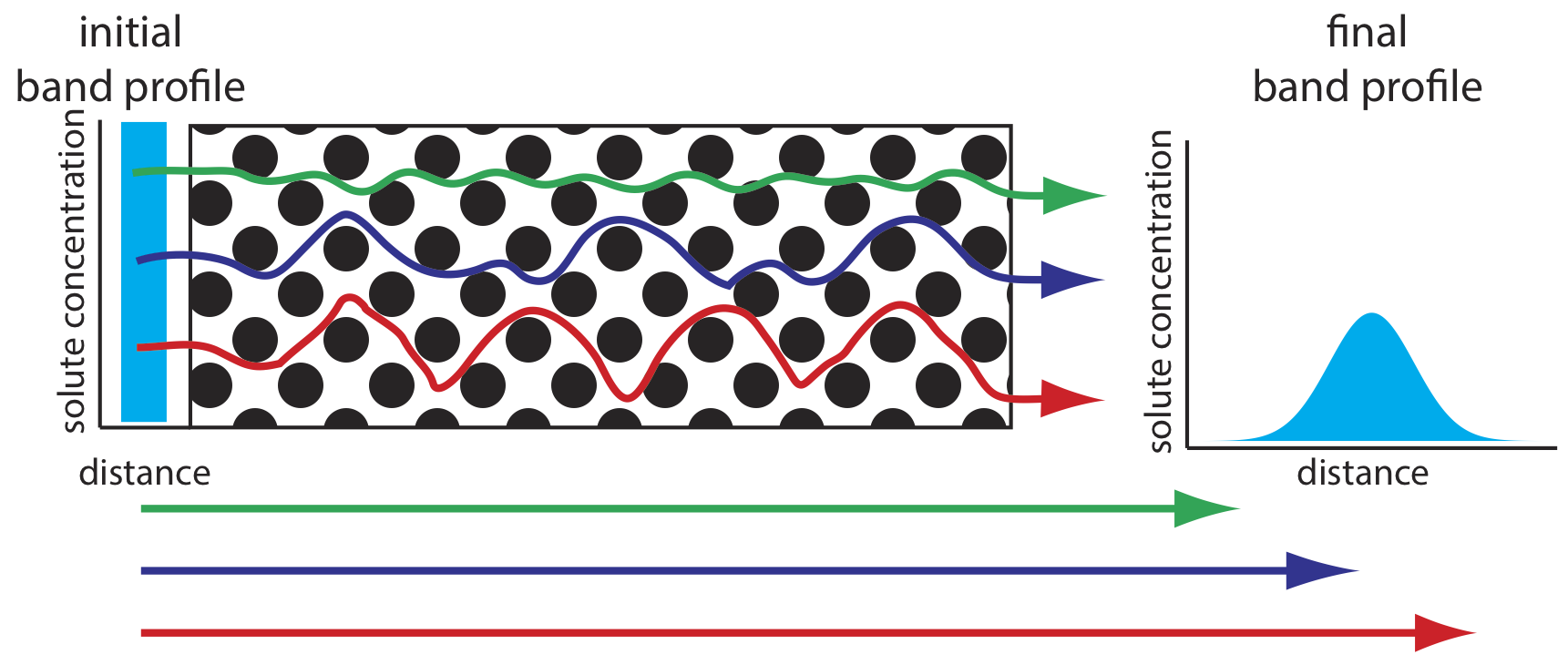
As solute molecules pass through the column they travel paths that differ in length. Because of this difference in path length, two solute molecules that enter the column at the same time will exit the column at different times. The result, as shown in Figure 12.3.4 , is a broadening of the solute’s profile on the column. The contribution of multiple paths to the height of a theoretical plate, H_p, is

\[H_{p}=2 \lambda d_{p} \label{12.5}\]

where d_p is the average diameter of the particulate packing material and \(\lambda\) is a constant that accounts for the consistency of the packing. A smaller range of particle sizes and a more consistent packing produce a smaller value for \(\lambda\). For a column without packing material, H_p is zero and there is no contribution to band broadening from multiple paths.

Figure 12.3.4 . The effect of multiple paths on a solute’s band broadening. The solute’s initial band profile is rectangular. As this band travels through the column, individual solute molecules travel different paths, three of which are shown by the meandering colored paths (the actual lengths of these paths are shown by the straight arrows at the bottom of the figure). Most solute molecules travel paths with lengths similar to that shown in blue, with a few traveling much shorter paths (green) or much longer paths (red). As a result, the solute’s band profile at the end of the column is broader and Gaussian in shape.

An inconsistent packing creates channels that allow some solute molecules to travel quickly through the column. It also can creates pockets that temporarily trap some solute molecules, slowing their progress through the column. A more uniform packing minimizes these problems.

Longitudinal Diffusion

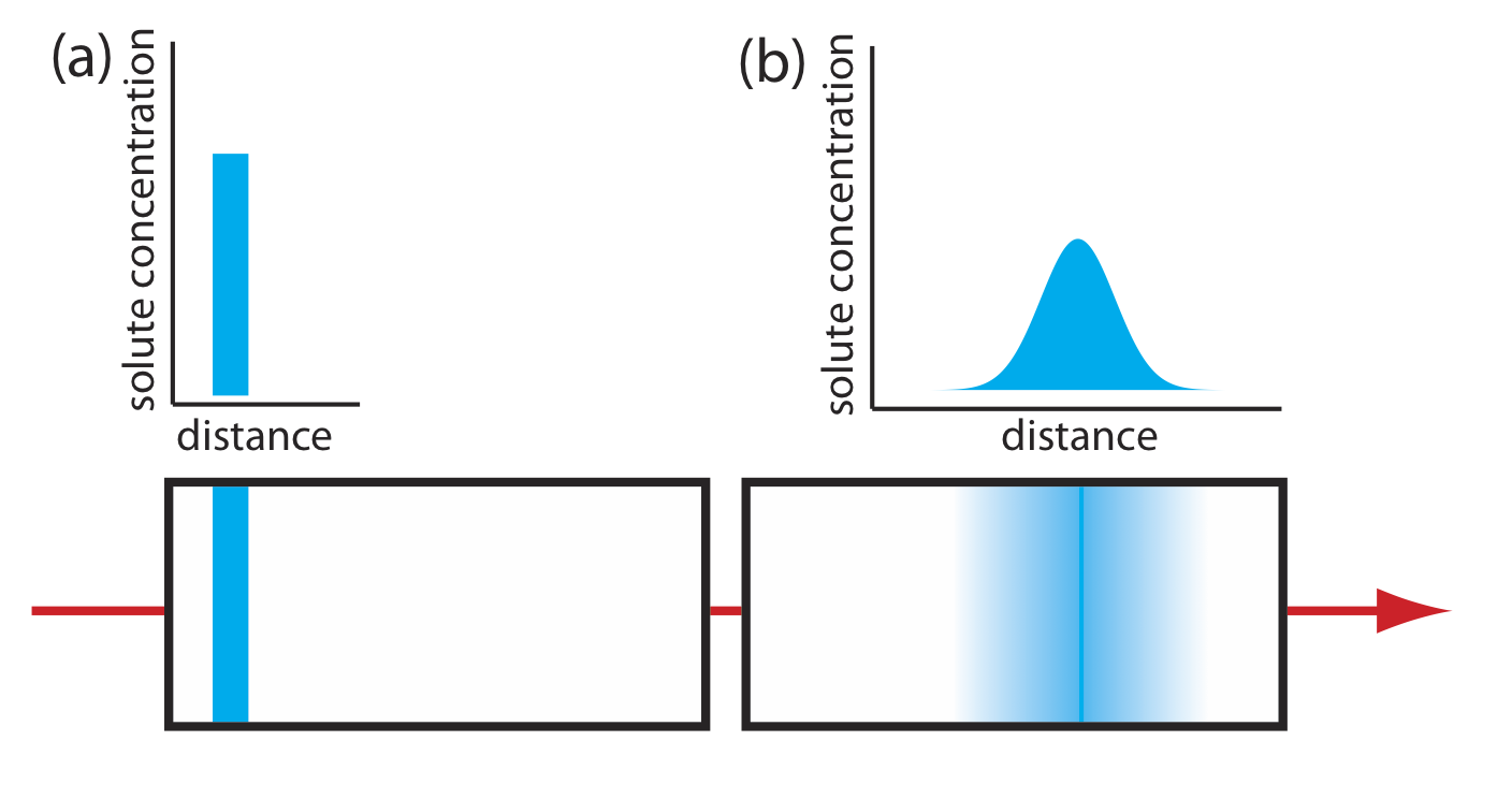
The second contribution to band broadening is the result of the solute’s longitudinal diffusion in the mobile phase. Solute molecules are in constant motion, diffusing from regions of higher solute concentration to regions where the concentration of solute is smaller. The result is an increase in the solute’s band width (Figure 12.3.5 ). The contribution of longitudinal diffusion to the height of a theoretical plate, H_d, is

\[H_{d}=\frac{2 \gamma D_{m}}{u} \label{12.6}\]

where D_m is the solute’s diffusion coefficient in the mobile phase, u is the mobile phase’s velocity, and \(\gamma\) is a constant related to the efficiency of column packing. Note that the effect of H_d on band broadening is inversely proportional to the mobile phase velocity: a higher velocity provides less time for longitudinal diffusion. Because a solute’s diffusion coefficient is larger in the gas phase than in a liquid phase, longitudinal diffusion is a more serious problem in gas chromatography.

Figure 12.3.5 . The effect of longitudinal diffusion on a solute’s band broadening. Two horizontal cross-sections through the column and the corresponding concentration versus distance profiles are shown, with (a) being earlier in time. The red arrow shows the direction in which the mobile phase is moving.

Mass Transfer

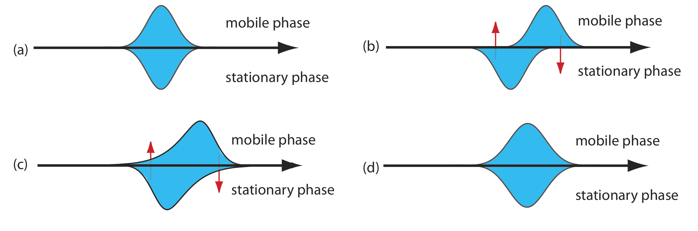
As the solute passes through the column it moves between the mobile phase and the stationary phase. We call this movement between phases mass transfer. As shown in Figure 12.3.6 , band broadening occurs if the solute’s movement within the mobile phase or within the stationary phase is not fast enough to maintain an equilibrium in its concentration between the two phases. On average, a solute molecule in the mobile phase moves down the column before it passes into the stationary phase. A solute molecule in the stationary phase, on the other hand, takes longer than expected to move back into the mobile phase. The contributions of mass transfer in the stationary phase, H_s, and mass transfer in the mobile phase, H_m, are given by the following equations

\[H_{s}=\frac{q k d_{f}^{2}}{(1+k)^{2} D_{s}} u \label{12.7}\]

\[H_{m}=\frac{f n\left(d_{p}^{2}, d_{c}^{2}\right)}{D_{m}} u \label{12.8}\]

where d_f is the thickness of the stationary phase, d_c is the diameter of the column, D_s and D_m are the diffusion coefficients for the solute in the stationary phase and the mobile phase, k is the solute’s retention factor, and q is a constant related to the column packing material. Although the exact form of H_m is not known, it is a function of particle size and column diameter. Note that the effect of H_s and H_m on band broadening is directly proportional to the mobile phase velocity because a smaller velocity provides more time for mass transfer.

The abbreviation fn in Equation \ref{12.7} means “is a function of.”

Figure 12.3.6 . Effect of mass transfer on band broadening: (a) Ideal equilibrium Gaussian profiles for the solute in the mobile phase and in the stationary phase. (b, c) If we allow the solute’s band to move a small distance down the column, an equilibrium between the two phases no longer exits. The red arrows show the movement of solute—what we call the mass transfer of solute—from the stationary phase to the mobile phase, and from the mobile phase to the stationary phase. (d) Once equilibrium is reestablished, the solute’s band is now broader.

Putting It All Together

The height of a theoretical plate is a summation of the contributions from each of the terms affecting band broadening.

\[H=H_{p}+H_{d}+H_{s}+H_{m} \label{12.9}\]

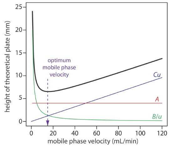
An alternative form of this equation is the van Deemter equation

\[H=A+\frac{B}{u}+C u \label{12.10}\]

which emphasizes the importance of the mobile phase’s velocity. In the van Deemter equation, A accounts for the contribution of multiple paths (H_p), B/u accounts for the contribution of longitudinal diffusion (H_d), and Cu accounts for the combined contribution of mass transfer in the stationary phase and in the mobile phase (H_s and H_m).

There is some disagreement on the best equation for describing the relationship between plate height and mobile phase velocity [Hawkes, S. J. J. Chem. Educ. 1983, 60, 393–398]. In addition to the van Deemter equation, other equations include

\[H=\frac{B}{u}+\left(C_s+C_{m}\right) u \nonumber\]

where C_s and C_m are the mass transfer terms for the stationary phase and the mobile phase and

\[H=A u^{1 / 3}+\frac{B}{u}+C u \nonumber\]

All three equations, and others, have been used to characterize chromatographic systems, with no single equation providing the best explanation in every case [Kennedy, R. T.; Jorgenson, J. W. Anal. Chem. 1989, 61, 1128–1135].

To increase the number of theoretical plates without increasing the length of the column, we need to decrease one or more of the terms in Equation \ref{12.9}. The easiest way to decrease H is to adjust the velocity of the mobile phase. For smaller mobile phase velocities, column efficiency is limited by longitudinal diffusion, and for higher mobile phase velocities efficiency is limited by the two mass transfer terms. As shown in Figure 12.3.7 —which uses the van Deemter equation—the optimum mobile phase velocity is the minimum in a plot of H as a function of u.

Figure 12.3.7 . Plot showing the relationship between the height of a theoretical plate, H, and the mobile phase’s velocity, u, based on the van Deemter equation.

The remaining parameters that affect the terms in Equation \ref{12.9} are functions of the column’s properties and suggest other possible approaches to improving column efficiency. For example, both H_p and H_m are a function of the size of the particles used to pack the column. Decreasing particle size, therefore, is another useful method for improving efficiency.

For a more detailed discussion of ways to assess the quality of a column, see Desmet, G.; Caooter, D.; Broeckhaven, K. “Graphical Data Represenation Methods to Assess the Quality of LC Columns,” Anal. Chem. 2015, 87, 8593–8602.

Perhaps the most important advancement in chromatography columns is the development of open-tubular, or capillary columns. These columns have very small diameters (d_c ≈ 50–500 μm) and contain no packing material (d_p = 0). Instead, the capillary column’s interior wall is coated with a thin film of the stationary phase. Plate height is reduced because the contribution to H from H_p (Equation \ref{12.5}) disappears and the contribution from H_m (Equation \ref{12.8}) becomes smaller. Because the column does not contain any solid packing material, it takes less pressure to move the mobile phase through the column, which allows for longer columns. The combination of a longer column and a smaller height for a theoretical plate increases the number of theoretical plates by approximately \(100 \times\). Capillary columns are not without disadvantages. Because they are much narrower than packed columns, they require a significantly smaller amount of sample, which may be difficult to inject reproducibly. Another approach to improving resolution is to use thin films of stationary phase, which decreases the contribution to H from H_s (Equation \ref{12.7}).

The smaller the particles, the more pressure is needed to push the mobile phase through the column. As a result, for any form of chromatography there is a practical limit to particle size.