2.3: Stoichiometric Calculations
- Page ID
- 127136
\( \newcommand{\vecs}[1]{\overset { \scriptstyle \rightharpoonup} {\mathbf{#1}} } \)
\( \newcommand{\vecd}[1]{\overset{-\!-\!\rightharpoonup}{\vphantom{a}\smash {#1}}} \)
\( \newcommand{\id}{\mathrm{id}}\) \( \newcommand{\Span}{\mathrm{span}}\)
( \newcommand{\kernel}{\mathrm{null}\,}\) \( \newcommand{\range}{\mathrm{range}\,}\)
\( \newcommand{\RealPart}{\mathrm{Re}}\) \( \newcommand{\ImaginaryPart}{\mathrm{Im}}\)
\( \newcommand{\Argument}{\mathrm{Arg}}\) \( \newcommand{\norm}[1]{\| #1 \|}\)
\( \newcommand{\inner}[2]{\langle #1, #2 \rangle}\)
\( \newcommand{\Span}{\mathrm{span}}\)
\( \newcommand{\id}{\mathrm{id}}\)
\( \newcommand{\Span}{\mathrm{span}}\)
\( \newcommand{\kernel}{\mathrm{null}\,}\)
\( \newcommand{\range}{\mathrm{range}\,}\)
\( \newcommand{\RealPart}{\mathrm{Re}}\)
\( \newcommand{\ImaginaryPart}{\mathrm{Im}}\)
\( \newcommand{\Argument}{\mathrm{Arg}}\)
\( \newcommand{\norm}[1]{\| #1 \|}\)
\( \newcommand{\inner}[2]{\langle #1, #2 \rangle}\)
\( \newcommand{\Span}{\mathrm{span}}\) \( \newcommand{\AA}{\unicode[.8,0]{x212B}}\)
\( \newcommand{\vectorA}[1]{\vec{#1}} % arrow\)
\( \newcommand{\vectorAt}[1]{\vec{\text{#1}}} % arrow\)
\( \newcommand{\vectorB}[1]{\overset { \scriptstyle \rightharpoonup} {\mathbf{#1}} } \)
\( \newcommand{\vectorC}[1]{\textbf{#1}} \)
\( \newcommand{\vectorD}[1]{\overrightarrow{#1}} \)
\( \newcommand{\vectorDt}[1]{\overrightarrow{\text{#1}}} \)
\( \newcommand{\vectE}[1]{\overset{-\!-\!\rightharpoonup}{\vphantom{a}\smash{\mathbf {#1}}}} \)
\( \newcommand{\vecs}[1]{\overset { \scriptstyle \rightharpoonup} {\mathbf{#1}} } \)
\( \newcommand{\vecd}[1]{\overset{-\!-\!\rightharpoonup}{\vphantom{a}\smash {#1}}} \)
\(\newcommand{\avec}{\mathbf a}\) \(\newcommand{\bvec}{\mathbf b}\) \(\newcommand{\cvec}{\mathbf c}\) \(\newcommand{\dvec}{\mathbf d}\) \(\newcommand{\dtil}{\widetilde{\mathbf d}}\) \(\newcommand{\evec}{\mathbf e}\) \(\newcommand{\fvec}{\mathbf f}\) \(\newcommand{\nvec}{\mathbf n}\) \(\newcommand{\pvec}{\mathbf p}\) \(\newcommand{\qvec}{\mathbf q}\) \(\newcommand{\svec}{\mathbf s}\) \(\newcommand{\tvec}{\mathbf t}\) \(\newcommand{\uvec}{\mathbf u}\) \(\newcommand{\vvec}{\mathbf v}\) \(\newcommand{\wvec}{\mathbf w}\) \(\newcommand{\xvec}{\mathbf x}\) \(\newcommand{\yvec}{\mathbf y}\) \(\newcommand{\zvec}{\mathbf z}\) \(\newcommand{\rvec}{\mathbf r}\) \(\newcommand{\mvec}{\mathbf m}\) \(\newcommand{\zerovec}{\mathbf 0}\) \(\newcommand{\onevec}{\mathbf 1}\) \(\newcommand{\real}{\mathbb R}\) \(\newcommand{\twovec}[2]{\left[\begin{array}{r}#1 \\ #2 \end{array}\right]}\) \(\newcommand{\ctwovec}[2]{\left[\begin{array}{c}#1 \\ #2 \end{array}\right]}\) \(\newcommand{\threevec}[3]{\left[\begin{array}{r}#1 \\ #2 \\ #3 \end{array}\right]}\) \(\newcommand{\cthreevec}[3]{\left[\begin{array}{c}#1 \\ #2 \\ #3 \end{array}\right]}\) \(\newcommand{\fourvec}[4]{\left[\begin{array}{r}#1 \\ #2 \\ #3 \\ #4 \end{array}\right]}\) \(\newcommand{\cfourvec}[4]{\left[\begin{array}{c}#1 \\ #2 \\ #3 \\ #4 \end{array}\right]}\) \(\newcommand{\fivevec}[5]{\left[\begin{array}{r}#1 \\ #2 \\ #3 \\ #4 \\ #5 \\ \end{array}\right]}\) \(\newcommand{\cfivevec}[5]{\left[\begin{array}{c}#1 \\ #2 \\ #3 \\ #4 \\ #5 \\ \end{array}\right]}\) \(\newcommand{\mattwo}[4]{\left[\begin{array}{rr}#1 \amp #2 \\ #3 \amp #4 \\ \end{array}\right]}\) \(\newcommand{\laspan}[1]{\text{Span}\{#1\}}\) \(\newcommand{\bcal}{\cal B}\) \(\newcommand{\ccal}{\cal C}\) \(\newcommand{\scal}{\cal S}\) \(\newcommand{\wcal}{\cal W}\) \(\newcommand{\ecal}{\cal E}\) \(\newcommand{\coords}[2]{\left\{#1\right\}_{#2}}\) \(\newcommand{\gray}[1]{\color{gray}{#1}}\) \(\newcommand{\lgray}[1]{\color{lightgray}{#1}}\) \(\newcommand{\rank}{\operatorname{rank}}\) \(\newcommand{\row}{\text{Row}}\) \(\newcommand{\col}{\text{Col}}\) \(\renewcommand{\row}{\text{Row}}\) \(\newcommand{\nul}{\text{Nul}}\) \(\newcommand{\var}{\text{Var}}\) \(\newcommand{\corr}{\text{corr}}\) \(\newcommand{\len}[1]{\left|#1\right|}\) \(\newcommand{\bbar}{\overline{\bvec}}\) \(\newcommand{\bhat}{\widehat{\bvec}}\) \(\newcommand{\bperp}{\bvec^\perp}\) \(\newcommand{\xhat}{\widehat{\xvec}}\) \(\newcommand{\vhat}{\widehat{\vvec}}\) \(\newcommand{\uhat}{\widehat{\uvec}}\) \(\newcommand{\what}{\widehat{\wvec}}\) \(\newcommand{\Sighat}{\widehat{\Sigma}}\) \(\newcommand{\lt}{<}\) \(\newcommand{\gt}{>}\) \(\newcommand{\amp}{&}\) \(\definecolor{fillinmathshade}{gray}{0.9}\)A balanced reaction, which defines the stoichiometric relationship between the moles of reactants and the moles of products, provides the basis for many analytical calculations. Consider, for example, an analysis for oxalic acid, H2C2O4, in which Fe3+ oxidizes oxalic acid to CO2
\[2\ce{Fe^{3+}}(aq) + \ce{H2C2O4}(aq) + 2\ce{H2O}(l) \ce{->} 2\ce{Fe^{2+}}(aq) + 2\ce{CO2}(g) + 2\ce{H3O+}(aq) \nonumber\]
The balanced reaction shows us that one mole of oxalic acid reacts with two moles of Fe3+. As shown in the following example, we can use this balanced reaction to determine the amount of H2C2O4 in a sample of rhubarb if we know the moles of Fe3+ needed to react completely with oxalic acid.
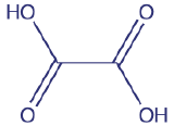
In sufficient amounts, oxalic acid, the structure for which is shown below, is toxic. At lower physiological concentrations it leads to the formation of kidney stones. The leaves of the rhubarb plant contain relatively high concentrations of oxalic acid. The stalk, which many individuals enjoy eating, contains much smaller concentrations of oxalic acid.

In the examples that follow, note that we retain an extra significant figure throughout the calculation, rounding to the correct number of significant figures at the end. We will follow this convention in any calculation that involves more than one step. If we forget that we are retaining an extra significant figure, we might report the final answer with one too many significant figures. Here we mark the extra digit in red for emphasis. Be sure you pick a system for keeping track of significant figures.
The amount of oxalic acid in a sample of rhubarb was determined by reacting with Fe3+. After extracting a 10.62 g of rhubarb with a solvent, oxidation of the oxalic acid required 36.44 mL of 0.0130 M Fe3+. What is the weight percent of oxalic acid in the sample of rhubarb?
Solution
We begin by calculating the moles of Fe3+ used in the reaction
\[\frac {0.0130 \text{ mol } \ce{Fe^{3+}}} {\text{L}} \times 0.03644 \text{ M} = 4.73{\color{Red} 7} \times 10^{-4} \text{ mol } \ce{Fe^{3+}} \nonumber\]
The moles of oxalic acid reacting with the Fe3+, therefore, is
\[4.73{\color{Red} 7} \times 10^{-4} \text{ mol } \ce{Fe^{3+}} \times \frac {1 \text{ mol } \ce{H2C2O4}} {2 \text{ mol } \ce{Fe^{3+}}} = 2.36{\color{Red} 8} \times 10^{-4} \text{ mol } \ce{H2C2O4} \nonumber\]
Converting the moles of oxalic acid to grams of oxalic acid
\[2.36{\color{Red} 8} \times 10^{-4} \text{ mol } \ce{H2C2O4} \times \frac {90.03 \text{ g } \ce{H2C2O4}} {\text{mol } \ce{H2C2O4}} = 2.13{\color{Red} 2} \times 10^{-2} \text{ g } \ce{H2C2O4} \nonumber\]
and calculating the weight percent gives the concentration of oxalic acid in the sample of rhubarb as
\[\frac {2.13{\color{Red} 2} \times 10^{-2} \text{ g } \ce{H2C2O4}} {10.62 \text{ g rhubarb}} \times 100 = 0.201 \text{% w/w } \ce{H2C2O4} \nonumber\]
You can dissolve a precipitate of AgBr by reacting it with Na2S2O3, as shown here.
\[\ce{AgBr}(s) + 2\ce{Na2S2O3}(aq) \ce{->} \ce{Ag(S2O3)_2^{3-}}(aq) + \ce{Br-}(aq) + 4\ce{Na+}(aq) \nonumber\]
How many mL of 0.0138 M Na2S2O3 do you need to dissolve 0.250 g of AgBr?
- Answer
-
First, we find the moles of AgBr
\[0.250 \text{ g AgBr} \times \frac {1 \text{ mol AgBr}} {187.8 \text{ g AgBr}} = 1.331 \times 10^{-3} \text{ mol AgBr} \nonumber\]
and then the moles and volume of Na2S2O3
\[1.331 \times 10^{-3} \text{ mol AgBr} \times \frac {2 \text{ mol } \ce{Na2S2O3}} {\text{mol AgBr}} = 2.662 \times 10^{-3} \text{ mol } \ce{Na2S2O3} \nonumber\]
\[2.662 \times 10^{-3} \text{ mol } \ce{Na2S2O3} \times \frac {1 \text{ L}} {0.0138 \text{ mol } \ce{Na2S2O3}} \times \frac {1000 \text{ mL}} {\text{L}} = 193 \text{ mL} \nonumber\]
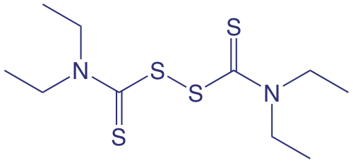
The analyte in Example 2.3.1 , oxalic acid, is in a chemically useful form because there is a reagent, Fe3+, that reacts with it quantitatively. In many analytical methods, we first must convert the analyte into a more accessible form before we can complete the analysis. For example, one method for the quantitative analysis of disulfiram, C10H20N2S4—the active ingredient in the drug Antabuse, and whose structure is shown below—requires that we first convert the sulfur to SO2 by combustion, and then oxidize the SO2 to H2SO4 by bubbling it through a solution of H2O2. When the conversion is complete, the amount of H2SO4 is determined by titrating with NaOH.

To convert the moles of NaOH used in the titration to the moles of disulfiram in the sample, we need to know the stoichiometry of each reaction. Writing a balanced reaction for H2SO4 and NaOH is straightforward
\[\ce{H2SO4}(aq) + 2\ce{NaOH}(aq) \ce{->} 2\ce{H2O}(l) + \ce{Na2SO4}(aq) \nonumber\]
but the balanced reactions for the oxidations of C10H20N2S4 to SO2, and of SO2 to H2SO4 are not as immediately obvious. Although we can balance these redox reactions, it is often easier to deduce the overall stoichiometry by use a little chemical logic.
An analysis for disulfiram, C10H20N2S4, in Antabuse is carried out by oxidizing the sulfur to H2SO4 and titrating the H2SO4 with NaOH. If a 0.4613-g sample of Antabuse requires 34.85 mL of 0.02500 M NaOH to titrate the H2SO4, what is the %w/w disulfiram in the sample?
Solution
Calculating the moles of H2SO4 is easy—first, we calculate the moles of NaOH used in the titration
\[(0.02500 \text{ M}) \times (0.03485 \text{ L}) = 8.712{\color{Red} 5} \times 10^{-4} \text{ mol NaOH} \nonumber\]
and then we use the titration reaction’s stoichiometry to calculate the corresponding moles of H2SO4.
\[8.712{\color{Red} 5} \times 10^{-4} \text{ mol NaOH} \times \frac {1 \text{ mol } \ce{H2SO4}} {2 \text{ mol NaOH}} = 4.356{\color{Red} 2} \times 10^{-4} \text{ mol } \ce{H2SO4} \nonumber\]
Here is where we use a little chemical logic. Instead of balancing the reactions for the combustion of C10H20N2S4 to SO2 and for the subsequent oxidation of SO2 to H2SO4, we recognize that a conservation of mass requires that all the sulfur in C10H20N2S4 ends up in the H2SO4; thus
\[4.356{\color{Red} 2} \times 10^{-4} \text{ mol } \ce{H2SO4} \times \frac {1 \text{ mol S}} {\text{mol } \ce{H2SO4}} \times \frac {1 \text{ mol } \ce{C10H20N2S4}} {4 \text{ mol S}} = 1.089{\color{Red} 0} \times 10^{-4} \text{ mol } \ce{C10H20N2S4} \nonumber\]
\[1.089{\color{Red} 0} \times 10^{-4} \text{ mol } \ce{C10H20N2S4} \times \frac {296.54 \text{ g } \ce{C10H20N2S4}} {\text{mol } \ce{C10H20N2S4}} = 0.03229{\color{Red} 3} \text{ g } \ce{C10H20N2S4} \nonumber\]
\[\frac {0.03229{\color{Red} 3} \text{ g } \ce{C10H20N2S4}} {0.4613 \text{ g sample}} \times 100 = 7.000 \text{% w/w } \ce{C10H20N2S4} \nonumber\]
A conservation of mass is the essence of stoichiometry!


