HPLC Retention Order

Exploring HPLC

Learning Objectives

After completing this exercise, students will be able to:

• Predict elution order of compounds
• Calculate retention factor and selectivity factor
• Explain the effect of mobile phase composition on resolution and peak shape at a molecular level
• Use elution gradients to improve separation of compounds in a mixture
• Explain the effect of flow rate on separation at a molecular level

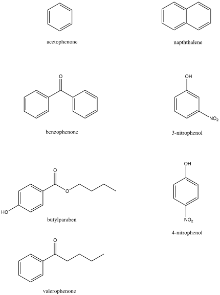
1. Consider the relative polarities of the following compounds:

2. Based on their structures and polarities, predict their retention order from least to most retained in RPLC. Write your prediction here:
   
   
   
   
   
    
3. Open the HPLC simulator (http://www.hplcsimulator.org/)
4. Confirm that the mobile phase flow rate is at 2.0 ml/min and the temperature is at 25 ^oC. Set the solvent to 50% acetonitrile.
5. Remove all of the compounds currently populating the compound list under the chromatogram.
6. Add acetophenone to the list at a concentration of 50 μmolar.

   Note its retention time: __________

   Note the void time: ___________

   Write the equation for retention factor here:

   
    

   Calculate the retention factor of acetophenone: ___________

   Compare it to the one listed in the table under the chromatogram.  

   Do they agree?______
    

7. Now add all of the other compounds above, one at a time, recording the retention factor for each as you add them.
   
   
   
   
   
   
   
   
   
    
8. Now change the solvent to 50% methanol. Record the retention factors for each compound in the table in your notebook.
   
   
   
   
   
   
   
    
9. By inspecting the retention factors you recorded, which mobile phase additive is stronger (i.e., make solutes elute faster), methanol or acetonitrile?
   
   
   
    
10. Are all the compounds well separated?
    
     
11. Use the organic modifier slider bar to add more water to the mobile phase (i.e., decrease the percent methanol). Keep increasing the percent water until the solutes are baseline resolved.

    Note following;

    Percent methanol:_________________  Percent water: ________________

                   

    Retention time and retention factor of 3-nitrophenol ___________,____________

                   

    Retention time and retention factor of 4-nitrophenol ___________,____________

 

12. Calculate the selectivity factor, α, for the two compounds.
    
    
    
    
     
13. Now change the mobile phase to 100% acetonitrile. Use the organic modifier slider bar to add more water to the mobile phase (i.e., decrease the percent ACN). Keep increasing the percent water until the solutes are baseline resolved.

    Note following;

    Percent ACN:_________________  Percent water: ________________

    Retention time and retention factor of 3-nitrophenol ___________,____________

    Retention time and retention factor of 4-nitrophenol ___________,____________

 

14. Calculate the selectivity factor, α, for the two compounds
    
    
    
     
15. Comparing the results from methanol and acetonitrile, if you were working in a laboratory in which you had to quantify 3-nitrophenol and 4-nitrophenol in hundreds of samples day after day, which of the final compositions that you noted above for MeOH and ACN would you use? Explain your choice:
    
    
    
     
16. Based on your selection, set the mobile phase appropriately. Describe the changes in peak height and shape that you see with differences in retention time. Explain these differences on a molecular level.
    
    
    
    
    
    
    
    
     
17. What is the problem called? How is it typically corrected?
    
    
     
18. Note the retention time of the longest retained compound.
    
     
19. Can you modify the simulation to obtain sharp peaks for all compounds? Do so. (Note you can add the solvent composition plot to the chromatogram in the plot options tab.) What conditions are used?
    
    
    
    
     
20. Note the retention time of the longest retained compound. In addition to sharpness of peaks, what additional benefit is derived from your new procedure?
    
     
21. Create a gradient that retains sharp peaks but lowers the overall retention time further.
    
    
    
    
    
    
     
22. Change the flow rate back and forth from 1.0 mL/min to 10.0 mL/min and look at the chromatograms. Describe the changes and explain the molecular level phenomenon that are causing the changes.
    
    
    
    
    
    
    
    
    
     
23. At a flow rate of 4.0 mL/min, find conditions that again get the peaks baseline resolved.
    
    
    
    
    
    
    
    
    
     

 

 

Metaanalysis of assignments

1. Describe in your own words the RP-HPLC concepts covered in each of the exercises you conducted. What major concepts were focused on in each assignment, and what, specifically, did you learn about each of those concepts. Take your time.  Review and think carefully about everything you did. 
   
   
   
   
   
   
    

Instructor Comments.

Here are some notes about this exercise using the HPLC simulator.  The entire assignment can be done as homework, but I found that it works well to do the first part as a class activity.  The students are asked to play with the fraction of organic solvent, ø, and to observe the influence that it has on the chromatogram of five compounds.  What conditions give the best resolution?

The next task is to come up with a model that will reliably predict the retention of a compound as a function of ø.  We assume that if a model works well for two compounds, it will apply to the others also.  The students work with one other person to record the retention factor, k’, as a function of ø from 20% to 80%.  They can very easily generate a plot of k' vs. ø with a spreadsheet and use the regression feature to find what sort of equation best fits the data.  My experience was that some people accepted a poor fit after a hasty guess, however, they were quickly persuaded by other students that an exponential expression (k'=ae^-bø) works best.   That provided an opportunity to talk about scrutinizing graphical models and minimizing residuals.

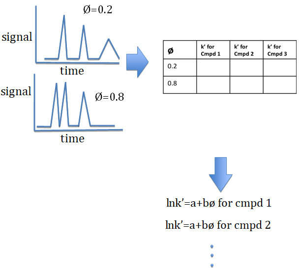
I gave them three different models to consider, but I'm not sure that was necessary.  However, I do think that it is a lot easier to work with the logarithmic version, lnk' = a + bø.  It’s intuitively friendlier and algebraically easier to find the slope and intercept for a linear equation for each compound using the data from only two chromatograms.

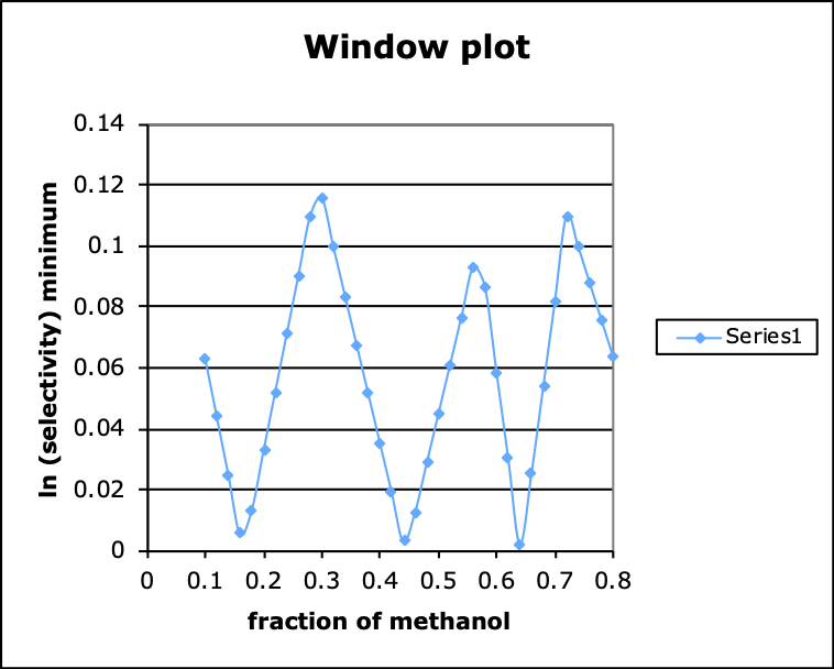
The remaining part of the exercise involves finding the optimum conditions for the best resolution.  (It is based on a graphical strategy called “window analysis” developed by Laub and Purnell [J. Chromatogr. 1975, 112, 71; Anal. Chem. 1976, 48, 799] for mixed stationary phases in GC and later applied to optimizing mobile phases in LC by Deming [J. Chromatogr. 1980, 199, 317].)  I gave this part as a homework assignment.  Once they have the specific equation for each compound, the students can quickly generate a table that calculates lnk' for each compound for an organic fraction from ø = 0.1 to 0.8 in steps of 0.02.  In each row (corresponding to a specific value of ø) the two values that are numerically most similar indicate which two compounds are the least well separated under those conditions. The students are asked to create a final column that takes the difference for that one pair. Of course, this is equivalent to the logarithm of the separation factor, α. This is a little bit tedious, since one must visually inspect 40 different rows separately.   A graph of this column vs. ø produces triangular windows.  The tops of these triangles coincide with conditions where the separation factors are highest for the most difficult-to-separate pair.  Going back to the HPLC simulator the students can try the optimum conditions and get the satisfaction of seeing the peaks baseline resolved.

ø	cmpd1	cmpd2	cmpd3	cmpd4	cmpd5	Min.
	lnk’	lnk’	lnk’	lnk’	lnk’	Lnk’1-lnk’2

HPLC Simulator Homework

Before viewing the simulator, attempt to answer the following question.  These questions are based on using liquid chromatography for the analytical separation of phenol, acetophenone, and p-nitrotoluene.

1. a) Draw the structures of three compounds. b) List them in the order of least polar to most polar.

 

2. What order would you expect these compounds to elute on a C-18 column?

 

3. How would you expect the elution times for these molecules to change if the mobile phase was adjusted from 100% water to 50% (%v/v) acetonitrile to 100% (%v/v) acetonitrile?

 

4. What would you expect to happen to the theoretical plate height if:
   1. the flow rate was increased significantly (2.0 mL/min to 6.0 ml/min) ?
   2. the diameter of the packing particles was increased (3.0 μm to 6.0 μm)
   3. the length of the column is doubled (100 mm to 200 mm)

 

5. How would the chromatogram be affected in each of above scenarios?

 

 

 

 

Go to the website: www.hplcsimulator.org

• Edit the compound list at the bottom of the screen to contain only the three compounds given above.
• Use the simulator to make the adjustments mentioned above. How does the provided chromatogram match your prediction?

 

 

 

 

 

 

 

Window Analysis for HPLC

Go on line and open the HPLC simulator at www.hplcsimulator.org.  Remove the default compounds and enter these compounds and their concentrations on the list for the simulator below the graph.

Acetophenone (20 µM); 3-phenyl propanol (25 µM); methyl benzoate (20 µM); anisole (30 µM); p-nitrobenzyl chloride (35 µM) using methanol as the organic modifier.

Part 1.

Adjust the mobile phase composition until you get baseline resolution between all of the compounds in your mixture.  Note the fraction, ø, of the organic solvent that corresponds to this chromatogram.

Unfortunately, finding the optimum conditions for separating a real mixture takes much more time (and solvent) in the lab.  However, we might save some time and effort, if we were able to predict the retention factors for each compound under different solvent conditions.  Use the simulator to gather some data.  We are going to mathematically model the retention as a function of solvent composition.  For now, focus on the two compounds that are currently the first and the third compounds on the list for your mixture. In Excel create a table for the retention factor, k', for both compounds at each solvent composition, ø, from 20% organic modifier to 80% organic modifier in steps of 10%. (In the table enter ø in decimal form, that is, ø = %organic modifier/100.) Create a graph of k’ vs. ø for both compounds.  Which of the following mathematical models appears to fit the relationship best for k’ as a function of ø?  (Fit the data for both compounds separately before deciding.)

1. k’ = a  +  bø
2. lnk’ =  a  +  bø
3. k’ =  aø²  +  bø  +  c

Part 2.

Return to the HPLC simulator and find the corresponding values for k’ for each of the three other compounds for 20 % organic modifier and 80 % organic modifier.  Estimate the parameters (a, b, c) for the model that you have decided best relates k’ to ø for these compounds. (Notice that by knowing the general form of the model, this data can be estimated from results from just two chromatograms.)

The mathematical model will let us predict the behavior of these compounds at other solvent conditions.  This could save time in running the real chromatograms in the lab.   Imagine that we want to resolve all of the components in this mixture isocratically.  Use the terms for the equations that you determined above. Calculate estimates for lnk’ for each of these compounds for ø from 0.1 to 0.8 in steps of 0.02 and enter them into a new table.

Next, at each value of ø calculate ABS(lnk₂-lnk’₁) for the closest pair of values for lnk’.  (Notice that this is equivalent to calculating the log of the selectivity factor, ln(α) = ln(k’₁/k’₂) for the least well-separated peaks at the corresponding value of ø.)  For convenience let’s call this term the selectivity.  On a new chart plot the selectivity vs ø (connecting the points with a smooth curve). This process produces a diagram called a window plot.  Each triangle in the diagram (thinking of the baseline as one side of each triangle) defines a window. The oblique sides of the window indicate the value for the selectivity for the least well-separated peaks in the chromatogram at those solvent conditions.  The apex of the tallest peak indicates conditions where the resolution is likely to be the best.

Do the conditions that you noted in the very first part of this exercise coincide with the top of one of the windows? Are there other windows that predict good resolution? If so, run the simulator again under those conditions.  Are all of the peaks well resolved?

If more than one set of conditions will produce a chromatogram with baseline resolution for all components in your mixture, what other considerations should be used in deciding the optimum operating conditions?  This analysis considers only the separation factor.  What other characteristics affect the resolution?

 

 

 

 

 

 

 

 

 

 

 

1. On the course website near the link for this problem set there is a link to a web-based HPLC simulator that is quite sophisticated in terms of functionality (www.hplcsimulator.org).  Choose analytes phenol, 3-phenyl propanol, acetophenone, p-chlorophenol, and p-nitrotoluene initially (these are the defaults), and set the temperature to 30 °C.  Now choose acetonitrile as the organic solvent, and adjust ϕ, the fraction of organic solvent in the mobile phase to 0.48.  Clicking on a compound name in the property table will highlight the chromatogram for the pure component in the chromatogram window.  Adjust the mobile phase composition until you get baseline resolution between acetophenone and p-chlorophenol, and record the value of ϕ at that point.  Now change ϕ significantly (higher or lower) until you see the peaks for acetophenone and p-chlorophenol overlap; keep adjusting ϕ until one peak effectively moves through the other and you get baseline resolution of the pair again, and record this value.  What causes this dramatic change in the relative shifting of these peaks?  What implications does this have for the optimization of separations of mixtures of compounds?
    
2. Use the HPLC simulator to come up with ‘rules of thumb’ for the following scenarios.  In each case, systematically vary the solvent type or composition and build a table of retention factors for three or four solutes as a function of the variable you change.  Then, use those data to build your statement.
   1. When changing the fraction of acetonitrile in the mobile phase over a relatively small range (e.g., 30%), decreasing the acetonitrile by ____________% increases retention by a factor of ____________.
   2. When changing from methanol to acetonitrile as the organic component of the mobile phase, approximately ____________% more/less acetonitrile must be used to obtain a retention factor similar to that obtained when using methanol.

 

 

 

 

 

 

 

 

 

3. To answer the following questions, access the HPLC simulator at www.hplcsimulator.org. In each case, present your results along with an explanation of your observations that is supported by theory.

   Before beginning, set the following parameters:

   Vol. Inj. – 0.1 μL

   Time Constant  – 0.01 s

   Offset – 0.1 munits

   Noise – 0.01

   1. Vary the flow rate from low (say 0.3 mL/min) to high (say 3 mL/min). What happens to the retention times, resolution and peak height? For a peak which is not badly overlapping any other peak, plot the peak height (from baseline to the apex) vs. flow rate. Explain the fundamental basis of the trend you observe.  What are the practical consequences of this relationship?
   2. Set the flow rate to 1 mL/min and vary the particle size from 1.8 to 3.5 then 5 microns. What happens to the retention times, resolution, peak height, and backpressure?   Explain your observations in terms of peak broadening theory.
   3. Set the particle size to 5 microns. Vary the column length from 5 to 10 to 15 cm. What happens to the retention times, resolution, peak height, and backpressure? Explain your observations in terms of peak broadening theory.

 

 

 

 

 

 

 

 

 

 

 

Contributors and Attributions

• Leonard Demoranville ([e-mail]) and Daniel Scott ([e-mail]), Centre College
• Modified from Mark F. Vitha, http://www.hplcsimulator.org/resources/index.php
• Sourced from the Analytical Sciences Digital Library