
12: Complex Coupling
- Page ID
- 332812

\( \newcommand{\vecs}[1]{\overset { \scriptstyle \rightharpoonup} {\mathbf{#1}} } \)
\( \newcommand{\vecd}[1]{\overset{-\!-\!\rightharpoonup}{\vphantom{a}\smash {#1}}} \)
\( \newcommand{\dsum}{\displaystyle\sum\limits} \)
\( \newcommand{\dint}{\displaystyle\int\limits} \)
\( \newcommand{\dlim}{\displaystyle\lim\limits} \)
\( \newcommand{\id}{\mathrm{id}}\) \( \newcommand{\Span}{\mathrm{span}}\)
( \newcommand{\kernel}{\mathrm{null}\,}\) \( \newcommand{\range}{\mathrm{range}\,}\)
\( \newcommand{\RealPart}{\mathrm{Re}}\) \( \newcommand{\ImaginaryPart}{\mathrm{Im}}\)
\( \newcommand{\Argument}{\mathrm{Arg}}\) \( \newcommand{\norm}[1]{\| #1 \|}\)
\( \newcommand{\inner}[2]{\langle #1, #2 \rangle}\)
\( \newcommand{\Span}{\mathrm{span}}\)
\( \newcommand{\id}{\mathrm{id}}\)
\( \newcommand{\Span}{\mathrm{span}}\)
\( \newcommand{\kernel}{\mathrm{null}\,}\)
\( \newcommand{\range}{\mathrm{range}\,}\)
\( \newcommand{\RealPart}{\mathrm{Re}}\)
\( \newcommand{\ImaginaryPart}{\mathrm{Im}}\)
\( \newcommand{\Argument}{\mathrm{Arg}}\)
\( \newcommand{\norm}[1]{\| #1 \|}\)
\( \newcommand{\inner}[2]{\langle #1, #2 \rangle}\)
\( \newcommand{\Span}{\mathrm{span}}\) \( \newcommand{\AA}{\unicode[.8,0]{x212B}}\)
\( \newcommand{\vectorA}[1]{\vec{#1}} % arrow\)
\( \newcommand{\vectorAt}[1]{\vec{\text{#1}}} % arrow\)
\( \newcommand{\vectorB}[1]{\overset { \scriptstyle \rightharpoonup} {\mathbf{#1}} } \)
\( \newcommand{\vectorC}[1]{\textbf{#1}} \)
\( \newcommand{\vectorD}[1]{\overrightarrow{#1}} \)
\( \newcommand{\vectorDt}[1]{\overrightarrow{\text{#1}}} \)
\( \newcommand{\vectE}[1]{\overset{-\!-\!\rightharpoonup}{\vphantom{a}\smash{\mathbf {#1}}}} \)
\( \newcommand{\vecs}[1]{\overset { \scriptstyle \rightharpoonup} {\mathbf{#1}} } \)
\(\newcommand{\longvect}{\overrightarrow}\)
\( \newcommand{\vecd}[1]{\overset{-\!-\!\rightharpoonup}{\vphantom{a}\smash {#1}}} \)
\(\newcommand{\avec}{\mathbf a}\) \(\newcommand{\bvec}{\mathbf b}\) \(\newcommand{\cvec}{\mathbf c}\) \(\newcommand{\dvec}{\mathbf d}\) \(\newcommand{\dtil}{\widetilde{\mathbf d}}\) \(\newcommand{\evec}{\mathbf e}\) \(\newcommand{\fvec}{\mathbf f}\) \(\newcommand{\nvec}{\mathbf n}\) \(\newcommand{\pvec}{\mathbf p}\) \(\newcommand{\qvec}{\mathbf q}\) \(\newcommand{\svec}{\mathbf s}\) \(\newcommand{\tvec}{\mathbf t}\) \(\newcommand{\uvec}{\mathbf u}\) \(\newcommand{\vvec}{\mathbf v}\) \(\newcommand{\wvec}{\mathbf w}\) \(\newcommand{\xvec}{\mathbf x}\) \(\newcommand{\yvec}{\mathbf y}\) \(\newcommand{\zvec}{\mathbf z}\) \(\newcommand{\rvec}{\mathbf r}\) \(\newcommand{\mvec}{\mathbf m}\) \(\newcommand{\zerovec}{\mathbf 0}\) \(\newcommand{\onevec}{\mathbf 1}\) \(\newcommand{\real}{\mathbb R}\) \(\newcommand{\twovec}[2]{\left[\begin{array}{r}#1 \\ #2 \end{array}\right]}\) \(\newcommand{\ctwovec}[2]{\left[\begin{array}{c}#1 \\ #2 \end{array}\right]}\) \(\newcommand{\threevec}[3]{\left[\begin{array}{r}#1 \\ #2 \\ #3 \end{array}\right]}\) \(\newcommand{\cthreevec}[3]{\left[\begin{array}{c}#1 \\ #2 \\ #3 \end{array}\right]}\) \(\newcommand{\fourvec}[4]{\left[\begin{array}{r}#1 \\ #2 \\ #3 \\ #4 \end{array}\right]}\) \(\newcommand{\cfourvec}[4]{\left[\begin{array}{c}#1 \\ #2 \\ #3 \\ #4 \end{array}\right]}\) \(\newcommand{\fivevec}[5]{\left[\begin{array}{r}#1 \\ #2 \\ #3 \\ #4 \\ #5 \\ \end{array}\right]}\) \(\newcommand{\cfivevec}[5]{\left[\begin{array}{c}#1 \\ #2 \\ #3 \\ #4 \\ #5 \\ \end{array}\right]}\) \(\newcommand{\mattwo}[4]{\left[\begin{array}{rr}#1 \amp #2 \\ #3 \amp #4 \\ \end{array}\right]}\) \(\newcommand{\laspan}[1]{\text{Span}\{#1\}}\) \(\newcommand{\bcal}{\cal B}\) \(\newcommand{\ccal}{\cal C}\) \(\newcommand{\scal}{\cal S}\) \(\newcommand{\wcal}{\cal W}\) \(\newcommand{\ecal}{\cal E}\) \(\newcommand{\coords}[2]{\left\{#1\right\}_{#2}}\) \(\newcommand{\gray}[1]{\color{gray}{#1}}\) \(\newcommand{\lgray}[1]{\color{lightgray}{#1}}\) \(\newcommand{\rank}{\operatorname{rank}}\) \(\newcommand{\row}{\text{Row}}\) \(\newcommand{\col}{\text{Col}}\) \(\renewcommand{\row}{\text{Row}}\) \(\newcommand{\nul}{\text{Nul}}\) \(\newcommand{\var}{\text{Var}}\) \(\newcommand{\corr}{\text{corr}}\) \(\newcommand{\len}[1]{\left|#1\right|}\) \(\newcommand{\bbar}{\overline{\bvec}}\) \(\newcommand{\bhat}{\widehat{\bvec}}\) \(\newcommand{\bperp}{\bvec^\perp}\) \(\newcommand{\xhat}{\widehat{\xvec}}\) \(\newcommand{\vhat}{\widehat{\vvec}}\) \(\newcommand{\uhat}{\widehat{\uvec}}\) \(\newcommand{\what}{\widehat{\wvec}}\) \(\newcommand{\Sighat}{\widehat{\Sigma}}\) \(\newcommand{\lt}{<}\) \(\newcommand{\gt}{>}\) \(\newcommand{\amp}{&}\) \(\definecolor{fillinmathshade}{gray}{0.9}\)Complex Splitting Patterns in 1H NMR*
Review: Probability
The n+1 splitting rule comes from simple probability.
Explore probability using pennies or NMR CoinFlip Game (Azman & Esteb, J. Chem. Educ., 2016, 93 (8), pp 1478–1482)
- If you have a penny, how many possible states can you have (ie heads/tails)?
- If you toss this penny in the air, what is the statistical distribution of these states (ie how often will you get heads vs tails?)
- If you have two pennies, how many possible states can you have?
- If you toss two pennies in the air, what is the statistical distribution of these states?
- If you have three pennies, how many states can you have? What is the statistical distribution of these states?
* All spectra are either from SDBS (Japan National Institute of Advanced Industrial Science and Technology) or simulated.
Origins of the n+1 rule
Nuclear spins are impacted by the NMR instrument magnet. However, the neighboring nuclei also have a magnetic field (charged particle with spin will generate a magnetic field). Splitting (multiplicity) arises from the interaction of the magnetic spin states of the neighboring protons.
In the example below, the signal for the methyl (CH3) in ethyl benzene “feels” an increase in magnetic field by having both the spin states of the neighboring methylene (CH2) in alignment with the applied magnetic field. This signal also “feels” a decrease in magnetic field by having both the spin states of the neighboring CH2 opposed to the applied magnetic field. There are yet two other combinations that do not lead to a net increase or decrease in magnetic field “felt”.
The methylene CH2 also is impacted by the different spin states of the 3 protons on the methyl next to it.

- Predict the spin states for:
- CH-CH
- CH-CH2
- CH-CH3
Statistical Distribution of Spin States
Note that the ratio of the peak heights is what we would predict if we used statistics (1:3:3:1 and 1:2:1).
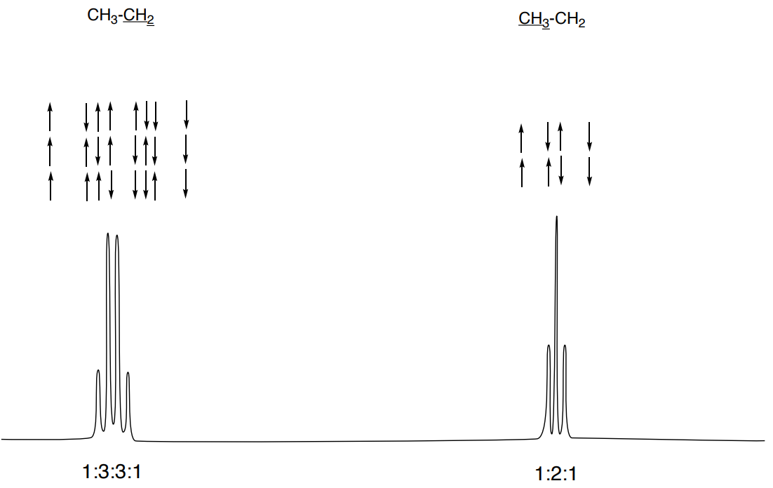
This ratio can be predicted with statistics or Pascal’s Triangle:

- How do you predict the next row in Pascal’s Triangle? Add it to the triangle above.
- What is the line shape for a quartet?
- Draw the line shape for a 7-line peak.
Introduction to Coupling Constants
The distance between any two adjacent lines in an NMR multiplet peak is called the coupling constant (symbol: J). This value is measured in Hz.

J coupling is mutual, i.e. JAB = JBA always.

The distance between the lines of a multiplet depends on the operating frequency of the spectrometer, but J (Hz) does not.
To convert the distance in ppm, into the coupling constant, multiply the distance by the operating frequency, expressed in MHz, of the NMR spectrometer used for the experiment.
- You have a 300 MHz NMR instrument. If the distance between the lines of your doublet was 0.025 ppm, what is the coupling constant (J)?
Typical Coupling Constant for alkanes (free rotation): 6-8 Hz
Practice Measuring Coupling Constants
The coupling constant must be the in two peaks that are coupled to each other. In the spectrum below, measure the coupling constants


- Assign all peaks in this spectrum to the compound drawn.
- Determine the coupling constants for each peak.
- Which two peaks are coupled to each other?
- Which peak is really a set of two singlets?
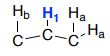
Splitting with Non-Equivalent Hydrogens
In the following structure, the blue hydrogen to appear as a triplet.

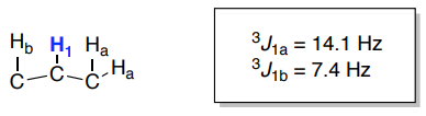
This peak only appears as a triplet if J1-a and J1-b are identical. When one of the hydrogens has a much bigger coupling constant, a complex coupling pattern is present.
In this case, the middle hydrogen can observe proton a and proton b both up or both down. This matches the triplet case seen earlier.
However, when one of the protons is up and the other down, they do not cancel out because they are not the same size. Now, four equivalent lines are shown.
This is called a doublet of doublets (dd).

- Using arrows and probabilities, predict the splitting patterns for the following systems. Assume that the coupling to Hb is larger than Ha.
- doublet of triplets (dt)
- doublet of quartets (dq)

- doublet of triplets (dt)
Splitting Trees to Analyze Complex Coupling
A good illustration of using splitting trees is provided by the 1H-NMR spectrum of methyl acrylate.

Consider the Hc signal, which is centered at 6.21 ppm.
Hc is coupled to both Ha and Hb , but with two different coupling constants.
A splitting diagram (or tree diagram) can help us to understand what we are seeing.
Ha is trans to Hc across the double bond and splits the Hc signal into a doublet with a coupling constant of 3Jac = 17.4 Hz. Each Hc doublet sub-peaks is split again by Hb (geminal coupling) into two more doublets with a much smaller coupling constant of 2Jbc = 1.5 Hz.

Splitting Trees to Analyze Complex Coupling (cont.)
The signal for Hb at 5.64 ppm is split into a doublet by Ha, a cis coupling with 3Jab = 10.4 Hz. Each of the resulting sub-peaks is split again by Hc, with the same germinal coupling constant 2Jbc = 1.5 Hz that we saw previously when we looked at the Hc signal.
The overall result is again a doublet of doublets, this time with the two `sub-doublets` spaced slightly closer due to the smaller coupling constant for the cis interaction. Here is a blow-up of the actual Hb signal:

- Construct a splitting diagram for the Hb signal in the 1H-NMR spectrum of methyl acrylate using the coupling constants provided.

The signal for Ha at 5.95 ppm is also a doublet of doublets.
- Construct a splitting diagram for the Ha signal in the 1H-NMR spectrum of methyl acrylate using the coupling constants provided.
Practice Splitting Diagrams with Complex Coupling:
- Construct a splitting diagram for Hn in each of the following cases.
- Name the coupling pattern. It is customary to put the larger coupling first and then the smaller coupling.
a.

b.

c.
Practice Recognizing Coupling Patterns
- Identify the coupling patterns shown below. Draw a splitting tree for each coupling pattern.


Practice Complex Coupling:

- Assign all peaks in this spectrum to the hydrogens in the compound shown above.
- Construct a splitting diagram for the peak at 4.2 ppm.
Structures that Exhibit Complex Coupling
Complex coupling is observed when there are non-equivalent hydrogens vicinal to the observed atom.
There are several situations when complex coupling is observed such as cyclohexane chairs, alkenes, long-range coupling, and chiral systems.
Systems with Complex Coupling: Rigid Systems
Coupling constants (distance between the peaks) vary when there is NOT free rotation.
Typical Coupling Constants:
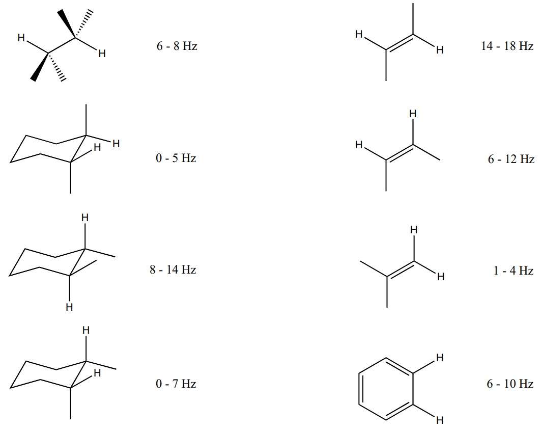
Coupling Constants Based on Angles: Karplus Relationship
When there is limited rotation in a structure, the coupling constant is dependent upon the dihedral angle between the two protons.
The Karplus relationship is based on the observation:
- Coupling is largest when the protons are at 180° or 0° dihedral angles (anti or eclipsed relationship results in optimal orbital overlap).
- Coupling will be close to 0 for protons that are 90° from each other.
While there are some variations based on substituents, the Karplus curves are generally reliable.
- Using the Karplus curve, what would you predict for 3J of the following structures?
- anti Hs on a Newman projection
- axial-axial on a chair
- axial-equatorial on a chair
- equatorial-equatorial on a chair

Systems with Complex Coupling: Diastereotopic Hydrogens
The concept of diastereotopicity was first introduced during the early days of NMR spectroscopy, when chiral molecules gave unexpectedly complex NMR spectra.
Nair, P. M.; Roberts, J. D. J. Am. Chem. Soc., 1957, 79, 4565
Diastereotopic protons are most commonly seen when a CH2 group are seen in a chiral molecule. These two seemingly equivalent protons will act as if they are nonequivalent.
For example, the beta CH2 of amino acids is next to the chiral alpha carbon and will be diastereotopic.
Phenylalanine 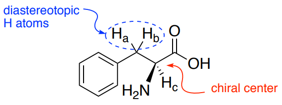
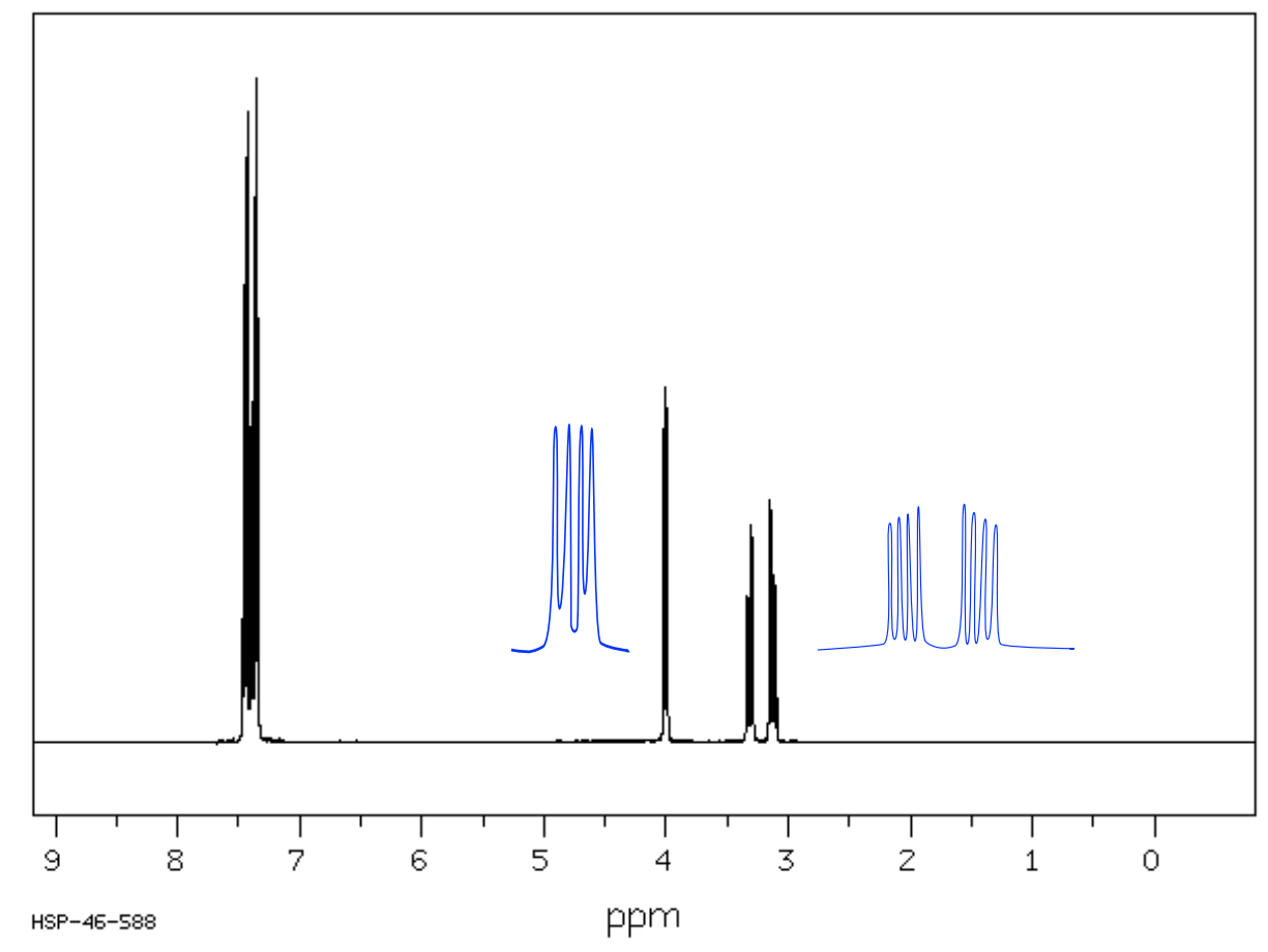
- What is the splitting pattern for each of the hydrogen atoms on this structure?
- Ha
- Hb
- Hc
Systems with Complex Coupling: Diastereotypic Hydrogens (cont.)
Diastereotopicity can also be seen when there are two equivalent methyl groups in a molecule with a chiral center.
- The NMR spectrum of 3-methyl-2-butanol is shown below. Identify the diastereotopic signals.

However, the CH2 groups in chiral molecules will NOT be diastereotopic if there is an axis of symmetry through the CH2 group.

- Predict whether the circled atoms would be diastereotopic:

Systems with Complex Coupling: Long-Range Coupling
Chem. Rev. 1977, 77, 599
Proton-proton couplings over more than three bonds are usually too small to detect easily (< 1 Hz) so they are not usually noticed. However, there are a number of important environments where these couplings are larger.
Coupling across \(\pi\)-systems are the most frequently encountered 4J couplings:
- meta-coupling in aromatic compounds

- 4-bond allylic and propargylic couplings

- "W-Coupling"

- 5J and higher are also observed in acetylenes
Practice:
1. The spectral data of cis-3-chloroacrylonitrile and trans-3-chloroacrylonitrile (C3H2NCl) is provided below.
- Draw the two isomers.
- Match each compound with the corresponding spectral information based on the coupling constants.
| Ha 5.8 ppm (J=14.0 Hz) | Ha 5.85 ppm (J=7.5 Hz) |
| Hb 7.12 ppm (J=14.0 Hz) | Hb 7.00 ppm (J=7.5 Hz) |
Miller & Kalnins, Tetrahedron, 1967, 23, 1145.
2. For acrylonitrile (shown below), assign the peaks.

- Analyze the following spectrum.
- Calculate coupling constants.
- Determine coupling pattern (dd, dt, q, etc.)
- Assign peaks to the hydrogens of the structure.
Note: On vinylic systems, protons on the same carbon (geminal) are not identical!

| Proton | JHH | Multiplicity |
|---|---|---|
| Ha |
a-b= a-c= |
|
| Hb |
b-c= b-a= |
|
| Hc |
c-b= c-a= |
3. Predict the proton NMR spectrum for trans-cinnemaldehyde. Use the table of coupling constants to predict J values also (using the table a few pages earlier).

| Proton | Shift | Multiplicity | JHH |
|---|---|---|---|
| Ha | d | a-b=6-7 | |
| Hb | dd |
b-c= b-a= |
|
| Hc | c-b= |
- How would the spectrum of cis-cinnemaldehyde differ?
| Proton | Shift | Multiplicity | JHH |
|---|---|---|---|
| Ha | d | a-b=6-7 | |
| Hb | dd |
b-c= b-a= |
|
| Hc | c-b= |
4. An organic chemistry student ran a hydroboration/oxidation reaction on 1- methylcyclohexene to form the product (2-methylcyclohexanol) for their independent synthesis.
- Draw the product: 2-methylcyclohexanol.
As this student continued her analysis, she realized that she might have different stereoisomers of 2-methylcyclohexanol.
- Draw the most stable conformation of cis-2-methylcyclohexanol.
- Draw the most stable conformation of trans-2-methylcyclohexanol.
The NMR spectra of cyclohexane structures can be difficult to interpret because of the overlapping peaks. However, the signal that corresponds to the H on the carbon bearing the hydroxyl group is very easy to pick out!
- What would you predict for the chemical shift of this hydrogen?
Practice 4. Cont.
The NMR coupling constant of the proton on the hydroxyl bearing carbon is a function of the dihedral angle between the hydrogens that are coupling to each other.
Remember, the coupling of these peaks can be more complicated than just simply a “sextet”! You may have a doublet of triplets, if two neighboring protons couple to this hydrogen in exactly the same way but a third one is different.

- Determine whether the student got cis-2-methylcylohexanol or trans-2-methylcylohexanol for the product. A table of coupling constants is on the following page. Show your work.
Summary
- What causes n+1 coupling?
- What causes complex coupling?
- What is a coupling constant? How do you measure it?
- What is a splitting tree?
- Show a splitting tree for a ddt (J = 3, 6, 12 Hz )
- What types of structural features display complex coupling patterns?
Spectral Problems with Complex Coupling
1. Propose a structure using the following data. Fully explain the complex coupling in the proton nmr.
MF: C4H6O SU:_____________

| Frequency | Functional Group |
|---|---|

Problem 1 (cont)

- Analyze the peaks from the 1H NMR of compound.
- Report them in the standard format (δ 0.00, dqt, J = 0.0, 0.0, 0.0, 2H).
- Provide part structure(s) defined by these protons. Underline the H observed.
| δ 3.61 ppm ______________________ | |
| δ 2.7 ppm ______________________ | |
| δ 2.27 ppm ______________________ | |
| δ 1.89 ppm ______________________ | |
| Proposed Structure: |
2. C4H6O SU = _____________
| Frequency | Functional Group |
|---|---|
| 3100 | |
| 2950 | |
| 2750 & 2875 | |
| 1700 | |
| 1650 | |
| 975 |

Problem 2 (cont)
1H NMR (expansions of peaks in blue)

| Chemical Shift | Integration | Multiplicity | Interpretation |
|---|---|---|---|
|
Proposed Structure*: Use IR and 1H NMR coupling to identify stereochemistry |
3.

MF:_______________ SU:_____________

| Frequency | Functional Group |
|---|---|
Problem 3 (cont)


| Chemical Shift | Integration | Multiplicity | Interpretation |
|---|---|---|---|